Aug 19, 1991 - A. van der Meulen,' Nico J. van Sittert,2'3 Adriaan ...... Jansen AP, Van Kampen EJ, Leynse B, Meyers CAM, Van ... Scand J Cliii Lab Invest.
CUN. CHEM.39/7, 1375-1381 (1993)
General Approachto Correctionfor Bias in AnalyticalPerformancein Longitudinal Studies Illustratedby Estimatingthe Effectof Age on y-GlutamyltransteraseActivity Egbert A. van der Meulen,’ Roe) van Strik’
Nico J. van Sittert,2’3
Adriaan
For studying trends in blood biochemistry analytes of an individual or a group of individuals, the outcome may be influenced by analytical changes that may have occurred during the study. An observed trend may well represent a drift in analytical performance instead of a truly biological finding. We developed a model that allows for retrospective correction of analytical changes with time. This model is based on the concept of adjustment of an indMdual’s longitudinal blood biochemistry data by comparing the long-term results of the laboratory with those of other laboratories in an external quality-controlsurvey program. Factors responsible for the analytical bias of our laboratory were identified by multiple regression analysis. The resulting procedure for assessing analytical bias and variability was applied to study in two mutually exclusive cohorts of employees of the Shell petrochemical complex in Rotterdam (a) the true nature of the changes (analytical or biological) in y-glutamyftransferase (GGT) and (b) the effect of age on GGT. The first cohort consisted of employees who attended a periodic health assessment in 1984 and in 1989; the second, employees who attended periodic health assessments in 1985 and in 1988. Thus we studied 3- and 5-year changes of GGT corrected for analytical bias. Whereas standard cross-sectional results apparently showed an increase of GGT up to age 50 years, the longitudinal findings corrected for analytical changes, as indicated above, do not support these cross-
sectional results. Indexing Terms: intra-Indwidualvariation
age-related effects enzyme activity variation, source of multiple regression analysis longitudinalvs cross-sectional studies .
For studying changes with time in blood biochemistry analytes measured in individual subjects, it is essential to correct for long-term analytical deviation in each individual’s data record. Short- and long-term analytical variation, or analytical imprecision, is usually assessed in internal (intra-) laboratory quality-control programs with use of quality-control specimens, either commercially freeze-dried survey serum or a frozen serum pooi (1-5), to monitor the analytical process. 1Department of Epidemiolor and Biostatistics, Erasmus University Medical School, The Netherlands. 2Biomedical Laboratory, Occupational Health Department
Shell Nederland
Raffinaderjj B.V./Shell Nederland Chexnie B.V., Rotterdam, The Netherlands. ‘Health, Safety and Environment Division, Shell Internationale Petroleum Maatschappij, P.O. Box 162, 2501 AN The Hague, The Netherlands (address correspondence to this author at this
address). Received August
19, 1991; accepted December
21, 1992.
G. J. de Koningh,2
Dick Lugtenburg,1
and
Long-term participation in external (inter-) laboratory quality-control programs permits the comparison of analyte concentrations with those measured in other laboratories using the same method, allowing the assessment of inaccuracy, or analytical bias, of the analyte under consideration (6, 7). Such data can also be used
for the retrospective
adjustment
of an individual’s
lon-
gitudinal blood biochemistry data. This is important to ensure that an observed trend with time represents a truly
biological
change
and not a drift in analytical
performance. In the Netherlands an external quality-control survey program, in which our laboratory participates, has been in operation since 1974 (6). In the present study, we have used the results for )-glut.amyltransferase (GOT) activities measured in quality-control serum, obtained from the organizers of this program over the period October 1983-June 1990, to investigate which determinants are responsible for the analytical bias in our laboratory. The resulting model, which allows for the assessment of analytical bias, is applied for the retrospective adjustment of GOT determinants in blood specimens (a) of employees of the Shell petrochemical complex collected during periodic health assessments in 1984 and 1989 and (b) of employees, not belonging to the previous cohort, of the same petrochemical complex collected during periodic health assessments in 1985 and 1988. We then used the adjusted GOT values, along with their analytical variability, to investigate whether the changes of serum GOT occurring in these 3 or 5 years were due only to analytical variation or to biological variation as well. Apart from studying the nature of the changes, we studied the influence of age, alcohol consumption, and body mass index on our GOT determinations corrected for analytical bias, both in longitudinal and cross-sec-
tional data. Materials
and Methods
The Quality-ControlProgram During the period of study (October 1983 to June 1990), -200 laboratories in The Netherlands participated in an external quality-control program (6). With bimonthly frequency, two different samples of qualitycontrol survey serum (one normal and one abnormal), either from human or animal source, were sent in freeze-dried form by the organizers to each of the participating laboratories for analyses of substrate concentrations and enzyme activities on a single day. The findings of each laboratory were reported to the organizers and, in return, the organizers reported to each CUNICAL CHEMISTRY, Vol. 39, No. 7, 1993
1375
participating laboratory the overall mean for all laboratory results of an analyte and also the mean for all laboratories using the same method For serum enzyme assays only the latter is relevant, because of the large differences between results obtained by difmethods to measure enzyme activity. During the period of study, our laboratory analyzed 80 quality-control specimens (40 normal and 40 abnor-
y,x
1,4
March 1. 1986
1,2
systematic
:
ferent
mal). Here we focus only on the findings of the determination of GOT in these 80 quality-control samples. The results from two samples analyzed during the period May 21 to July 13, 1984, were discarded, because a separate internal quality-control program (8) revealed that during this period the analytical CV of daily analyses of a quality-control sample was above the pre-set acceptance limit of 5%. This left a total of 78 GOT values from quality-control samples from the external quality-control program. We denote the value of GOT measured by our laboratory as x1 and the mean of all measurements made by the other -50 laboratories using the same method as y. This mean value y is regarded as the “true” value, with which we compare our laboratory result x1. The means Yi, y75 are shown in Figure 1. Figure 2 displays the performance of our laboratory as expressed by the ratios yjx1,, (i = 1, 78). As shown, the ratio changed on March 1, 1985, presumably because of a change in the analytical instrument we used (see below). ...,
GGT Assay GOT was determined carboxy-4-nitroanilide
at 30#{176}C with L-y-gluthmyl-3(2.9 mmol/L) as a substrate. In
1983, 1984, and in January/February determined with a programmable (PABOO; Vitatron Since
Scientific,
1985, GOT was
discrete analyzer The Netherlands).
Dieren,
1, 1985, GOT analyses
March
out with a Hitachi 705 automated
have been
analyzer
carried
(Boehringer,
Mnnnheim, Germany). Fresh human serum specimens (normal and pathological; 54 total) were analyzed both with the PABOO (v) and the Hitachi 705 (u) to study the y X
‘:
,
:.
#{149}.#{149}.
is
S...
0,8 0,8
-
83
84
88
86
87
89
88
90
91
year
FIg. 2. Ratios (y,1x11,I
78) of the meanGOT values In
quality-control
by laboratories
= 1, ... serum determined
using the same
analytical method to the GGT measurements performed laboratory during the periodOctober 1983 to June 1990
correlation
ii
=
between 0.86v
by our
the two methods. The regression 3 (r = 0.999). Since the introduction of the Hitachi 705, the same GOT method has been used throughout the study period (Boehringer Mannheim; Dutch cat. nos. 543098 and 543101). line was
-
Model for AssessingAnalytical Bias and Variability To assessthe analytical bias of GOT values in qualitycontrol serum determined in our laboratory, we used a multiple linear regression analysis, in which the mean of the -50 laboratory values (y) constitutes the dependent variable and our laboratory measurement (x1) is one of the explanatory variables. The following characteristics of our laboratory were considered to be possible explanatory variables as well: x2: A dummy variable, which
takes account of a change in the analytical instrument on March 1, 1985. Its value isO for samples analyzed before this date and 1 for samples analyzed thereafter. x3, x4: Human or animal source of quality-control serum. Two dummies are needed here because in several cases the source was unknown (the organizers of the quality-control program have provided the source of the quality-control serum only since February 9, 1987). Herex3 refers to whether or not the source was known (1 = yes/0 = no); for those cases with known source, x4 indicates whether it was human or animal. x5,.
X
:
..#{149}.
.,x11:Dummiestoindicateinwhichyear(1983-
.
200
1989) the serum was measured. x12, x: Dummies to indicate
X
.
x
X X
XX
XX
XxX
X X
X
X
XXX
XX
84
X
XX
XXX X
X 83
X
x
X
X
X 88
87
88
X
X
89
90
year FIg. 1. Mean values for GGT (y,, I = 1, ..., 78) in quality-control serum reported by -50 laboratories using the same analytical method during the perIod October 1983 to June 1990 1376
CUNICAL CHEMISTRY, Vol. 39, No. 7, 1993
in which month the
...,
X
course, 86
.,
serum was measured. Because it is unlikely that analytical bias would be smoothly related (e.g., linearly) to either the calendar year or the month of measurement if ordered according to some conceivable parameters, e.g., average temperatare of month, such relationships were not considered. Although the dummy variables x5, X would, of
XX
X
x
100
.
.
be less powerful
in the detection
of, e.g., a
.
strictly linear ing departures
relationship,
they are powerful
in detect-
from the no-effect hypothesis, irrespective of their direction. Returning to a more general context, let us assume k
explanatory
(in our situation,
variables
we start with k Extendingthe Model to Human Serum
=
22). Then the model is
Suppose we are interested i=1,...,78
where e1,. e.8 denote the errors, which are assumed to be an independent random sample from the normal distribution with mean 0 and variance or2. 0r2 is constant, i.e., does not depend on the precise values of explanatory variables (homoscedasticity). A standard ordinary least-squares regression analysis provides the usual estimates b of f3 and the mean squared error s2 as an estimate of o. Naturally, in verifying these assumptions, note first of all that independence of e1, e8 is obvious (in the quality-control program, each serum is from a different human or animal source). The normality of the errors can be checked empirically by focusing on the residuals (y b0 bkxk,,, i = 1,. 78). The assumption of homoscedasticity can be verified by plotting residuals against predicted values (b0 + b1x1,1 + + bkxkP i = 1, 78) and visually checking whether variability of the residuals does not increase with increasing (or decreasing) predicted values. More formally, one may apply the test for heteroscedasticity as described by White (9). If this assumption is not valid-e.g., o-2 clearly increases with x1-one performs a variancestabilizing transformation on y, e.g., a natural logarithm transformation. The influence of each explanatory variable or set of explanatory variables is, as usual, assessed by means of appropriate F-tests, which indicate whether the reduction in mean squared error is statistically significant. This eventually leaves us a subset of the most relevant explanatory variables. For a hypothetically measured x1 of analyte, we are now in the position to estimate the median and the 2.5th and the 9 7.5th percentiles of the distribution of the random variable Y, the outcome of which is identified with y, the mean of (approximately) 50 fictitious laboratory measurements. These percentiles provide us a tolerance interval of “probable” values of y; we refer to them as an analytical-bias-corrected tolerance interval. The natural estimate of the mean of Y, given x1,. is9 = b0 + b1x1 #{247}+ bkxk. (Equivalently,9isthe best linear predictor ofy based onx1,. X,.) Just as the obvious estimate of the variance 0r2 (the conditional variance of Y, given x1, X,,) is the mean squared error s2, the natural approximation to the exact 95% tolerance interval (p0 + + P Xk 1.96o /3 + + Pk Xk + 1.96o) is (9 1.96s, 9 + 1.96s). However, if the sample size is small and (or) the values of the explanatory values of the new analyte are rather extreme with respect to those found in the regression analysis, the standard error (SE) of the estimate 9 of the (conditional) mean of Y may become large relative to the mean squared error 2, which itself is inaccurate as an estimate of 0r2 in the instance of a small sample size. In those situations, it is reasonable to enlarge the tolerance interval, e.g., by replacing s with s + SE(9). .
.,
.
-
-
..
.
-
.
.
.,
.,
...
...,
.
...
.
.,
...,
...
-
-
...
.,
in whether the difference
between two consecutive measurements on the same person can reasonably be supposed to be due to analytical variation only. It would be convenient if the model described in the previous subsection could be applied irrespective of whether quality-control serum or fresh human serum is used. If indeed this assumption is justified, we may proceed as follows. First, let z1 denote
the vector of explanatory ment and z2 the similar
variables
at the first measure-
vector at the second measurement. If the time between the two measurements is large, we can assume that the random variable Y1 (the outcome Yi of which is the mean of -50 fictitious first laboratory measurements of this particular serum) is
independent of the similarly defined random variable Y2 for the second measurement, at least conditionally, given z1 and z2. In this case, the variance of the difference (D = Y2 Y1, given z1 and z2) is simply 2cr2. The obvious estimate of the mean of D is = 92 -9i where 91 and 92 are the estimated means of Y1 and Y2 (given z1 and z2), respectively. Because the difference of two normal distributions is again normal, the approximate 95% tolerance interval for d = Y2 Yi is, under the assumption of (conditional) independence, 1.96 + 1.96 V’?). Note that if Y1 and Y2 are not independent, they most likely will be positively correlated, in which case the -
a
-
(a
\/,
-
a
above tolerance
interval
turns
out to be a conservative
one (i.e., with a probability >0.95%, d will be in the tolerance interval indicated). If 0 is not in the 95% tolerance interval (i.e., if it is unlikely that d will equal 0), the observed difference corrected for analytical bias cannot be ascribed to analytical variation only, but must be ascribed to biological variation
also.
Applicationto Cohortsof Shell Employees The analytical bias model has been applied to (a) male employees of the Shell petrochemical complex who attended two voluntary periodic health assessments, one in 1984 and one in 1989, and (b) employees who attended periodic health assessment in 1985 (not before March 1), and in 1988. Thus we studied 3- and 5-year intra-individual changes in GOT corrected for analytical bias. Because the analytical bias model does not apply for samples analyzed during the period May 21 to July 13, 1984, employees who attended a periodic health assessment during this period are excluded, leaving a total of 1019 employees for study a. Study b involves 432 employees, all of whom are different from those of study a.
The reasons for performing these cohort studies by the described in the previous sections are: 1) To illustrate the analytical bias model. The Result8 section shows that our laboratory results are on the average higher than the “true” values y in 1984, lower in 1985 (after March 1, 1985), and only slightly lower in 1988 and 1989. The analytical bias model is thus apmethodology
CLINICAL CHEMISTRY, Vol. 39, No. 7, 1993 1377
plied in two different situations: with respect to the 1984-1989 study, we have to correct for a decrease due to analytical bias; with respect to the 1985-1988 study, we have to correct for an increase due to analytical bias. 2) To study whether 3- and 5-year intra-individual changes in GOT corrected for analytical bias are or are not due to analytical variation only. 3) To study whether age, alcohol consumption, and (or) body mass index variables contain significant information regarding GOT corrected for the analytical bias. These three variables were shown to be important determinRnts of GOT in several cross-sectional studies (10-15). We were interested in whether these results would hold when viewed from a longitudinal perspective also. Our emphasis was on studying the effect of age; alcohol consumption and body mass index served primarily as possible confounders. In addition to the longitudinal studies indicated, we performed cross-sectional studies, so that we could compare longitudinal results with the corresponding cross-sectional results. Regression analyses were performed for determining the influence of age, body mass index, and alcohol consumption on GOT, both for the cross-sectional and the longitudinal studies (in the latter case the difference in log GOT value served as the dependent variable). Serum GOT measurements were carried out from blood samples collected between 0800 and 1000. The GOT activity was determined on the day of the blood collection by the analytical methods described previously. Alcohol consumption had been recorded by means of a questionnaire in 1985, 1988, and 1989, but not in 1984. Results Analytical Bias Model The first part of this study was directed variables that are relevant determinants
at identifying of analytical
bias. A preliminary regression analysis showed that the residuals were not normally distributed and that variability of the residuals increased with x1 (heteroscedasticity). These problems were obviated by a logarithmic
transformation
of both x1 andy.
Multiple-regression analysis of in Y on the possible determinants described earlier showed that hi x1, x2 (change in analytical instrument), x7 (1985), x5 (1986), and an interaction of in x1 and x2 were relevant determinants of analytical bias (reducing the mean squared error significantly: P