Apr 10, 2012 - six dimensional (2,0) AN theory on a Riemann surface with irregular singularities. ... Argyres-Douglas (AD) theories [6] whose Coulomb branch ...
arXiv:1204.2270v1 [hep-th] 10 Apr 2012
Preprint typeset in JHEP style - HYPER VERSION
General Argyres-Douglas Theory
Dan Xie School of Natural Sciences, Institute for Advanced Study Princeton, NJ 08540, USA
Abstract: We construct a large class of Argyres-Douglas type theories by compactifying six dimensional (2, 0) AN theory on a Riemann surface with irregular singularities. We give a complete classification for the choices of Riemann surface and the singularities. The Seiberg-Witten curve and scaling dimensions of the operator spectrum are worked out. Three dimensional mirror theory and the central charges a and c are also calculated for some subsets, etc. Our results greatly enlarge the landscape of N = 2 superconformal field theory and in fact also include previous theories constructed using regular singularity on the sphere.
Contents 1. Introduction
3
2. Generalities of Argyres-Douglas theory
5
3. Irregular singularity of Hitchin’s equation 3.1 Classification of irregular singularity
7 10
4. AD points from 6d A1 theory 15 4.1 The construction of AD points 16 4.1.1 One irregular singularity: (A1 , AN −1 ) SCFT 16 4.1.2 One irregular singularity, One regular singularity: (A1 , DN +2 ) SCFT 17 4.2 Three dimensional mirror 18 4.3 AD points from linear quiver 19 4.4 Central Charge a and c 20 4.5 More singularities: Gauge theory coupled with (A1 , DN +2 ) theory 22 5. AD points from 6d A2 theory 5.1 Classification of irregular singularity for AD theories 5.1.1 Type I SCFT: (A2 , AN −1 ) theory 5.1.2 Type II SCFT 5.1.3 Type III SCFT 5.1.4 Type IV: One regular singularity, One irregular singularity 5.2 Three dimensional mirror theory 5.3 Central charges a and c 5.4 AD theories from SU (3) QCD 5.5 The use of the type IV SCFT
23 23 25 27 27 28 29 30 31 32
6. AD points from 6d Ak−1 theory 6.1 The choices of irregular singularity 6.1.1 Type I SCFT: (Ak−1 , AN −1 ) theory 6.1.2 Type II SCFT 6.1.3 Type III SCFT 6.1.4 Adding one more regular singularity: Type IV SCFT 6.2 3d Mirror symmetry 6.3 Equivalence between SCFTs 6.3.1 Irregular representations for theories of class S 6.4 A conjecture for R(B) and central charges a and c 6.4.1 Confirmation from mirror symmetry 6.5 AD points from N = 2 QCD 6.6 General irregular singularities
32 32 35 37 37 38 39 41 42 44 45 46 47
–1–
7. Six dimensional representation of known examples
47
8. Conclusion
49
–2–
1. Introduction The study of conformal field theory (CFT) plays an important role in understanding the dynamics of quantum field theory. The most well known four dimensional CFT is N = 4 supersymmetric gauge theory which has a conformal manifold labeled by an exact marginal coupling τ : gauge coupling constant. The weakly coupled description with explicit Lagrangian description can be written down at the cusp of the coupling constant space. Different weakly coupled descriptions are related by S duality which is best understood from the magical six dimensional (2, 0) theory compactified on a torus [1]. Recently, a large class of four dimensional N = 2 superconformal field theories (SCFT) are found by compactifying six dimensional (2, 0) theory on a punctured Riemann surface [2, 3]. Similarly, the gauge coupling constant space is identified with the moduli space of complex structure of the punctured Riemann surface and the S duality is the modular group. However, one usually can not write a Lagrangian description for the weakly coupled gauge theory duality frame at the cusps. The reason is that the matter sector is usually isolated strongly coupled SCFT which plays an essential role in understanding S duality of these theories, for instance, the S dual theory of SU (3) with six fundamentals [4] involves strongly coupled E6 theory [5] which can be constructed by compactifying six dimensional A2 theory on a sphere with three full punctures. The above theories have dimensionless coupling constants and the Coulomb branch operators have integer scaling dimension. There are another class of N = 2 SCFTs called Argyres-Douglas (AD) theories [6] whose Coulomb branch parameters usually have fractional scaling dimensions and there is also dimensional coupling constant. This type of theory is originally found as the IR theory at special point of Coulomb branch of pure SU (3) gauge theory. At this point, mutually nonlocal dyons become massless and one can not go to a duality frame in which these dyons carry only electric charge. The theory must be an interacting SCFT [6, 7] and one could not write a Lagrangian for it. There are usually relevant operators appearing in the spectrum which can be used to deform the theories to a new fixed point. It is natural to ask whether we can engineer the AD theories using the six dimensional (2, 0) theory and encode all those physical properties into the geometric objects on the Riemann surface. The answer is yes and it is necessary to introduce new type of puncture to encode the dimensional coupling constant: irregular singularity (higher order pole) [3]. The previous analysis is based on A1 (2, 0) theory and we will carry a complete analysis for higher rank theory in this paper. It is immediately clear that the possibility for finding new theories are dramatically increased. It is amazingly simple to classify and study these theories once a six dimensional construction is found. In the following, we outline the main strategy of constructing AD theories and summarize the main results. The Hitchin equation defined on the Riemann surface [8, 9] plays a central role in these constructions. Let’s first review what happens in the regular puncture case. The four dimensional UV theory is specified by the boundary condition of the fields in the Hitchin’s equation at the puncture: they have the regular singularity (first order pole). The gauge coupling constant is the complex structure moduli of punctured Riemann surface, and the
–3–
mass parameters are encoded as the coefficients of the first order pole. The IR behavior of the four dimensional theory is determined by the moduli space of solutions with the above specified boundary condition. In particular, the Seiberg-Witten curve is identified with the spectral curve of the Hitchin integrable system. There is no way to introduce dimensional couplings using only regular punctures so the irregular singularity for the solution of Hitchin’s equation is needed. The introduction of the irregular singularity provides us the desired properties: first the operators of 4d theory have fractional scaling dimension; second the parameters in the higher order pole are the dimensional coupling constants. The coefficient in the first order pole is still identified with the mass parameter, therefore all the deformation parameters of the UV theory are matched with the geometric parameters. The moduli space has similar properties as the regular singularity case, i.e. it is also a hyperkahler manifold [10]. One can also identify the spectral curve of the moduli space with the Seiberg-Witten curve. So the IR behavior of the theory is solved too. The regular singularity is classified by Young Tableaux and one can put arbitrarily number of punctures on a Riemann surface with arbitrary genus to define a SCFT. The situation is completely different for the irregular singularity case. First, since the coordinate z of the Riemann surface transforms non-trivially under the 4d U (1)R symmetry, one can only use the the Riemann sphere to preserve the U (1)R symmetry. Second, there are also severe constraints on the combinations of irregular singularity and regular singularity one can put on a Riemann surface. Finally, the classification of irregular singularity is much more fruitful but not every irregular singularity defines an AD theory. To construct an AD theory, we have the following constraints: 1. Only Riemann sphere can be used. 2. There are two singularity combinations: a. Only one irregular singularity; b. One irregular singularity and one regular singularity. 3. There are only three classes of irregular singularities. By specifying the singularity structure on the Riemann sphere, one can write the spectral curve and therefore find the scaling dimensions of various operators appearing in the theory. The three dimensional mirror theory for some of the AD theories can also be determined from the information of the irregular singularity. The central charges a and c of those theories can be easily calculated using 3d mirror theory. The theories we constructed recover almost all the AD theories found in the literature and there are a lot more new examples. Not all the SCFTs constructed are distinct and we identify some of the interesting isomorphism which is useful in calculating the central charge of these theories, etc. By allowing the higher order pole, the possible choices for constructing SCFT are greatly increased even with the above constraints. Our results greatly enlarge the landscape of N = 2 SCFT and show that these AD theories are much more generic than people thought. In fact, the theory of class S (theory using regular singularity) defined on a sphere can also be realized using irregular singularity. Some more properties of these theories are also studied in this paper. First, we use the collision of the singularities to identify the AD points of the SU (N ) QCD which serves as a
–4–
possible UV completion of AD theories; Second, if the AD theory has one regular singularity which usually has non-abelian flavor symmetry, one can use this theory to construct new asymptotical free (AF) theory. Geometrically, such AF theories are engineered by putting arbitrary number of irregular singularities on a Riemann surface. This paper is organized as follows: in section 2, we give a brief review of AD theory; In section 3, an introduction and classification to irregular singularity of Hitchin’s equation are given; section 4 discusses the AD theory found from six dimensional A1 theory, and those theories are not new but we study various properties of these theories which seem new; In section 5, AD theories from A2 theory are classified and studied; section 6 consider the general AD theory found from compactifying six dimensional Ak−1 theory; Section 7 discuss the six dimensional construction of the known AD theories; finally, we give a short discussion showing possible further directions in section 8.
2. Generalities of Argyres-Douglas theory The Argyres-Douglas theory is first discovered as the IR theory at certain point of Coulomb branch of pure SU(3) gauge theory [6]. At this point, there are mutually non-local massless dyons so one can not go to a duality frame in which all the massless matters carry only electric charge, so a Lagrangian description is not possible. It is further argued that the theory must be an interacting SCFT based on the superconformal algebra [11]. Several more examples were also found on the Coulomb branch of SU (2) QCD by tuning the mass parameters and Coulomb branch parameters [11]. For example, the AD theory from SU (2) with only one flavor is the same as that found from pure SU(3) theory. The Seiberg-Witten curve of this theory is x2 = z 3 + mz + u.
(2.1)
The scaling dimension of the various operators are found by requiring the Seiberg-Witten differential λ = xdz to have dimension one: [x] + [z] = 1.
(2.2)
One also require that each term in the Seiberg-Witten curve to have the same dimension, therefore the scaling dimensions of coordinates x and z for the above theory are [x] = 35 and [z] = 25 . Then it is easy to find the scaling dimension [m] = 54 and [u] = 65 . u is a relevant operator and m is the coupling constant for this deformation, it is important to have [m] + [u] = 2 so the above interpretation of the deformation is possible. In fact, for any relevant operator ui of a AD theory, there has to be a coupling constant mi in the spectrum so that [ui ] + [mi ] = 2 [11]. The U (1)R charge of the operator is related to the scaling dimension at the superconformal point: R(ui ) = 2D(ui ). This U (1)R in the IR has nothing to do with the UV U (1)R symmetry, though.
–5–
(2.3)
It is interesting to note that the AD theory found in above examples has the same number of parameters as the UV theory, however, their scaling dimensions are changed dramatically due to the strong quantum effects. In some cases, even the Coulomb branch dimension is changed, for example, the above AD theory can also be found from pure SU (3) gauge theory, and the UV theory has Coulomb branch dimension 2 while the IR theory has Coulomb branch dimension one. Similarly, the flavor symmetry of the AD theory can be quite different from the UV theory. The above theory has no flavor symmetry, but there are other AD theories which carry non-abelian flavor symmetry, for example, the AD theory from the SU (2) with two flavors has a SU (2) flavor symmetry. Let’s list some of AD theories found in the literature: many more examples [12, 13] are found on the Coulomb branch of SU (N ) and SO(N ) QCD by tuning the parameters. The AD theories found from SU (2) QCD are labelled as A0 , A1 , A2 theory from singular fibre classification, the higher rank generalizations of them are found using F theory by putting multiple D3 branes at the singularity of the corresponding type [14, 15, 16]. Recently, a large class of theories based on a pair of Dynkin diagrams are found in [17] using the 2d/4d correspondence. See also recent investigations of AD theories using F theory in [18]. Now let’s introduce some of the important quantities associated to a N = 2 theory. The four dimensional superconformal field theories have two important central charges parameterizing the trace anomaly [19]: < Tµµ >=
a c (W eyl)2 − (Euler), 16π 2 16π 2
(2.4)
where 1 2 2 (W eyl)2 = Rµνρσ − 2Rµν + R2 , 3 2 2 (Euler) = Rµνρσ − 4Rµν + R2 .
(2.5)
For a weakly coupled N = 2 gauge theory, the central charge can be expressed as the number of vector multiplets nv and hypermultiplets nh [20]: c=
2nv + nh 5nv + nh , a= , 12 24 1 a−c= (nv − nh ). 24
(2.6)
Here the quantity a − c is proportional to the dimension of ”Higgs” branch in which all the gauge symmetry is broken, and this fact is important for our later calculation. There is another useful general equation for the central charge 4(2a − c) =
r X (2D(ui ) − 1).
(2.7)
i=1
It is very hard to calculate the central charge for strongly coupled theories. By using the topological gauge theory, the author of [20] found the following formula: 1 5 1 1 a = R(A) + R(B) + r + h, 4 6 24 24
–6–
1 1 1 c = R(B) + r + h, 3 6 12
(2.8)
where r is the number of vector multiplets at the generic point of the Coulomb branch and h is the free hypermultiplets at generic point; R(A) and R(B) are R charge of certain measure factors for the topological gauge theory. R(A) can be found from the scaling dimension of the Coulomb branch operators: X R(A) = (D(ui ) − 1). (2.9) i
and R(B) is related to the discriminant of Seiberg-Witten curve which is in general very difficult to calculate. The central charges can also be calculated using the supergravity dual [21].
3. Irregular singularity of Hitchin’s equation AD theories are constructed by compactifying six dimensional A1 theory on a Riemann surface with irregular singularity [3]. This is found by taking some scaling limit of the Seiberg-Witten curve of known UV theories and then map the resulting Seiberg-Witten curve to a Hitchin system description. The generalization of this method to higher rank theory is rather difficult and there are some subtle points about the scaling limit as discussed recently in [22]. Our philosophy is to start directly from the irregular singular solutions of Hitchin’s equation, and use the classification of irregular singularity to define a 4d theory. The same idea seems working well for the regular puncture case in which the solution of the Hitchin equation do have a Young Tableaux classification which matches the physical derivation [23]. It is clear that irregular singular solution (higher order pole) of Hitchin’s equation is needed for the AD theories if we require the matching between the UV parameters of the field theory and the geometric parameters. The new features of the AD theory are the fractional scaling dimension and the dimensional coupling constant, there is no way to accommodate these new features using only regular singularities. The introduction of the irregularity automatically solve this problem: first, the coordinate z on the Riemann surface transforms nontrivially and we have the fractional scaling; second, the coefficients in the higher order pole are the dimensional coupling constant. There are many other wonderful matchings between the geometric description and the physical quantities as we will discuss in full detail later. This section is mainly served as a description of the irregular singularity and those who want to see examples can skip this section in first reading. Let’s review various identifications between the physical quantities and the geometric aspects of Hitchin equation in more detail for the regular puncture cases which are later generalized to the irregular singularity case. The four dimensional N = 2 theory constructed in [2] are derived by compactifying six dimensional (2, 0) SCFT on a Riemann surface with regular punctures (with topological twist). The Hitchin’s equation is also defined on this Riemann surface and the punctures correspond to the regular singular solutions to Hitchin’s equation. The moduli space of solutions to Hitchin’s equation with fixed boundary condition is a hyperkahler manifold and is identified with the Coulomb branch of four dimensional theory on R3 × S 1 , where S 1 is a circle. In fact, the Hitchin moduli space
–7–
is the Higgs branch of the five dimensional maximal super Yang-Mills theory compactified on the punctured Riemann surface and it is the mirror of the original 3d theory [24]. There are no quantum corrections to the Higgs branch due to the non-renormalization theorem, that’s why the classical picture of the Hitchin equation encodes the Coulomb branch information of the original theory. The geometric parameters are the complex moduli of the punctured Riemann surface and the coefficients of the simple pole. The complex structure moduli is the gauge coupling constant while the coefficient of the simple pole is the mass parameter, so we identify all the UV deformation parameters of four dimensional theory. The IR behavior of the field theory is encoded into the moduli space which is a hyperkahler manifold with complex structures parametrized by CP 1 . In one of complex structure I, the Hitchin’s moduli space is an integrable system and the spectral curve is identified with the Seiberg-Witten curve. In complex structure J, each point on the moduli space parameterizes a flat connection on Riemann surface. Let’s discuss the Hitchin equation in some more detail. By taking a complex structure on the Riemann surface, the Hitchin equation reads F − φ ∧ φ = 0, Dφ = D ∗ φ = 0,
(3.1)
where A is the connection and φ is a one form called Higgs field [8, 25]. By writing A = A + iφ, the Hitchin equation implies that the curvature of A is flat. In fact, one can introduce a spectral parameter and define a family of flat connections depending on the spectral parameter. The monodromy around the singularity can be calculated by solving the following flat section equation: (∂z + Az )ψ = 0, (3.2) which locally is just a first order differential equation on the disk. Let’s now turn to irregular singular solution to Hitchin’s equation [26]. The simplest one with gauge group SU (N ) is φ=
un u2 u1 + ..... + 2 + + c.c + ...., n z z z A = αdθ.
(3.3)
Here we choose local coordinate z = reiθ , u1 , ...un are all diagonal matrix after using gauge symmetry, and they are regular semi-simple which means the eigenvalues are all different. The dot means the regular terms and we will ignore them in the formula below but they are always there. This abelianization of the Higgs field is crucial for finding the solution to irregular singular solution to Hitchin’s equation. If n = 1, setting u1 = β + iγ, then we have the solution with regular singularity: φ=β
dr − γdθ, r A = αdθ.
–8–
(3.4)
In fact, there is no need to take u1 regular semi-simple, the local solution is actually labeled by Young Tableaux with total boxes N. The spectral curve of the Hitchin integrable system is det(x − Φ(z)) = 0, (3.5) where Φ is the holomorphic part of the gauge field. This is identified as the Seiberg-Witten curve. Physically, The coefficient on the simple pole encodes the mass parameters while the gauge couplings depend on the positions of the pole. The identification of the mass with the coefficient of the simple pole is the following: the two form on the Seiberg-Witten geometry should depend linearly on the mass [27, 28] while the Hitchin moduli space in complex structure I do depend linearly on the coefficient of the simple pole [29]. The Hitchin moduli space in the presence of irregular singularities is also hyperkahler [10] and they share many properties as the regular singularity, in particular, the complex structure I depends linearly on the coefficient of the first order which should be identified with the mass parameter [26]. The complex structure J in which each point represents a flat connection is useful for many purposes and we will focus on it in the following. For the irregular singularity, the flat connection of this solution has the following form Az =
u2 α − iγ un un−1 + n−1 + .... 2 − i . zn z z z
(3.6)
There is an interesting Stokes phenomenon for the differential equation (3.2) which is important to define the monodromy around the irregular singularity. We will review some aspects for the Stokes phenomenon for the completeness, the interested reader can find more details in [26, 30]. The appearance of these Stokes matrices are coming from the asymptotical behavior of the solutions to the equation (∂ + Az )ψ = 0. Assume the gauge group is U(1), then the differential equation becomes dψ qn qn−1 q1 = −( n + n−1 ... + + B(z))ψ, dz z z z
(3.7)
here B(z) is a holomorphic function which is regular at z = 0. The solution is very simple: ψ = c(z) exp Q(z), qn qn−1 Q(z) = ( + ... + q1 (−lnz), (n − 1)z n−1 (n − 2)z n−2
(3.8)
c(z) is a formal power series which is not convergent around the singularity. This solution is the building block for the solution of the higher rank, which just have a vector of above solution with index i = 1, 2, ...n. However, the entries of solution vector have different asymptotical behaviors along different path to the singularity because |
qni − qnj exp Qi (z) | → | exp( )|, exp Qj (z) (n − 1)z n−1
z → 0. i
j
(3.9)
qn −qn The asymptotical behavior depends on the sign of Re( (n−1)z n−1 ). The sign is different for different angular region and it is easy to see that there are 2(n − 1) angular regions which are called Stokes sector, the boundary of the Stokes sector is called Stokes ray.
–9–
The point is the solution with given asymptotical behavior in a region is not unique if i (z)) there is no stokes ray. For example, if | exp(Q exp(Qj (z) )| >> 0 in this region, then the solution ′
ψi (z) = ψi (z) + λψj (z) has the same asymptotical behavior as ψi . Such freedom is not here if there is a Stokes ray in this angular region. Let’s take a region with angular width π/(n − 1) whose boundary is not a stokes ray. By rotating this region by integer value of π n−1 , we get a cover of the disk. One can enlarge each sector a little bit such that there is no stokes ray in the overlapping region. There will be a stokes ray for any given pair of entries in the solution vector in each sector and the whole solution is uniquely fixed with given asymptotical behaviors in that region. On the overlapping region,the two sets of solutions are related by an upper triangular matrix with unit diagonal entry. This matrix is called as the Stokes matrix which is then used to construct the monodromy matrices. There would be a total of 2(n − 1) stokes matrices and the product of them defines part of the generalized monodromy. The monodromy also has a contribution from the regular singular term which contribute a N − 1 parameter. Finally we need to subtract a contribution from the Tc group which has dimension (N − 1). So the total parameters in specifying the local monodromy is cn = (n − 1)(N 2 − N ).
(3.10)
The monodromy for a path around the irregular singularity with a chosen base point has another contribution which contributes an extra (N 2 −1) parameters. However, the moduli space is defined by specifying the leading order coefficient which gives a minus (N − 1) contribution. So the total contribution to the moduli space of the irregular singularity is d = n(N 2 − N ).
(3.11)
If there are more than one irregular singularity, the total dimension of the moduli space is the sum of local contribution minus a gauge group contribution X di − 2(N 2 − 1). (3.12) dim(M ) = i
The local contribution of the irregular singularity to the moduli space can also be understood in an easy way as the following [31]: each fixed regular semi-simple matrix defines a conjugacy glass Oi in the lie algebra. The differential operator dA maps one point from the product of n conjugacy class to a point on the moduli space of flat connections: dA : O1 × O2 × O3 . . . × On → M.
(3.13)
Since each regular semi-simple conjugacy class of Sl(N ) has dimension N 2 − N , the total dimension of the local contribution is d = n(N 2 − N ) which maps the result from the consideration of stokes matrices. 3.1 Classification of irregular singularity Let’s give a classification of irregular singularity in this subsection. The classification is achieved by specifying the matrices of of the higher order pole and it is easier by considering the application to field theory. We do not distinguish the difference between the
– 10 –
holomorphic part of the Higgs field and the contribution from the gauge field by assuming the first order pole coefficients of these two parts are in the same conjugacy class. By introducing ω = 1z , the equation (3.2) becomes dψ ′ = Φ (ω)ψ, dω ′ Φ (ω) = z −2 Φ(1/z).
(3.14)
Now the singularity is put at ω = ∞, and we use the singularity at 0 and ∞ in this paper interchangeably. The singularity at ∞ is good for classification and finding the Seiberg-Witten curve, while the choice 0 is good for considering the collision of irregular singularity. The key point is that the matrices specifying the behavior of the singularity can be put into diagonal form by using formal gauge transformation [26]. The classification for irregular singularity for our purpose is to specify the form of these diagonal matrices. The leading order matrix can have the following form Φ(z) = λdiag(z r1 −2 B1 , z r2 −2 B2 , . . . , z rs −2 Bs ),
(3.15)
here Bi is a ki × ki diagonal matrix whose eigenvalue degeneracy will be discussed later, and r1 ≥ r2 ≥ r3 . . . ≥ rs are a set of rational numbers denoting the order of pole of various blocks. The crucial point now is that the resulting spectral curve should have only integer power in z, therefore the rational number ri should be ri = ni +
ji , ki
0 < ji ≤ ki .
(3.16)
Now let’s study the degeneracy of eigenvalues of various matrices and we only need to consider just block B1 , the consideration is exactly same for the other blocks. If j1 6= k1 , the eigenvalues can only have the following form (assume j1 and k1 have no common divisor, the degeneracy case is considered later): B1 = diag(1, ω, ω 2 , . . . , ω k1 −1 ),
j1 6= k1
(3.17)
with ω = exp( 2πi k1 ), we do not write this value explicitly in later sections, but ω always have the above form with proper choice of k1 . The meaning of such fractional power Higgs field in the gauge theory context is explained in [26]: there is a cut coming out singularity and one need to do a gauge transformation to put the gauge field Φ(θ + 2π) back to Φ(θ). One can also do a gauge transformation to put the above solution into a non-singular one, but it is not good for our purpose and we will stick to the above exotic representation. If j1 = k1 , the pole ri is integer and the eigenvalues of Bi are all the same. B1 = diag(a, a, . . . , a),
j1 = k1 .
(3.18)
The sub-leading matrices are determined by requirement that every possible deformation compatible with leading order matrix is allowed: the same gauge transformation
– 11 –
we introduced earlier should transform it to its original value after circling around the singularity. If j1 = k1 , the next term also has integer order n1 − 1 whose matrix has eigenvalue degeneracy determined by a partition of k1 . Similarly, one need to specify all the lower order matrices by giving the degeneracy of the eigenvalues. The leading order matrix is not enough to completely specify the irregular singularity in the integer pole case. The only exception is that the dimension of this block is just one since there can be no degeneracy for one eigenvalue. The situation is different if j1 < k1 , in that case all the terms having the following form should be allowed z
m+ kl −2 1
(ω d , ω d+1 , ω d+2 , . . . , ω (k1 +d−1) ),
(3.19)
where m is an integer and (m + kl1 ) < r1 , and d is a fixed integer depending only on l, more detailed discussion on this can be found in [32]. Moreover, the following terms are also allowed it there are more than one block z m (a, a, . . . , a),
(3.20)
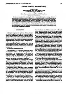
with m < r1 an integer. There is a nice graphic representation for the leading order matrices which turns out to be really useful to find the Seiberg-Witten curve. The irregular singularity is represented by a convex Newton polygon on a two dimensional integer lattice. The convex polygon is determined as following: first find a point p1 such that the slope of the line between p1 and point (N, 0) has slope r1 − 2. Then another point p2 is chosen such that the slope of the line p2 p1 has the value r2 − 2, etc. We have a convex polygon at the end. See figure. 1. The above graph is not enough to determine the irregular singularity if there is a segment with integer slope, one also need to specify the degeneracy of the matrices of the lower order pole. Here are some important examples: a. The irregular singularity considered in last subsection corresponds to r1 = . . . = rs = n with n an integer. Moreover, each block is one dimensional. The irregular singularity is completely fixed by the form of the leading order term. b. The leading order has partition [N − 1, 1]. This irregular singularity is also completely fixed by the leading order form Φ = z r−2 diag(0, 1, ω, . . . , ω N −2 ).
(3.21)
c. The leading order has partition [N ] or there is only one block in the leading order, the order of pole is fractional. d. We still have r1 = . . . = rs = n, but the leading order singularity is specified by a Young Tableaux Yn which represents the block structure of the leading order matrix. Then we need a collection of Young Tableaux such that Yn ⊆ Yn−1 . . . ⊆ Y1 , where Yj−1 is derived by further partitioning each column of the Yj . Notice that, the scenario a is the special case in which all the Young Tableaux have the form [1, 1, 1, . . . , 1]. More generally,
– 12 –
Figure 1: The Newton polygon representing an irregular singularity, each segment on the boundary represents a block and its slope is the order of pole of that block.
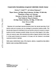
if there are integer points on the boundary of b and c, one can take a combination of the boundary dots and decompose this block into several smaller one, the irregular singularity is completely fixed by the leading order though. Notice that the four classes have one thing in common: the leading order matrix has the same order of pole, those irregular singularities are the one needed for defining the AD theories. Moreover, the leading order matrix of case a, b, c all have distinct eigenvalues. The case a, c can be represented by a Newton polygon as shown in the left of figure. 2 with appropriate dots on the boundary for a, and case b is represented on the right of figure.2.
Figure 2: Left: The Newton polygon for the irregular singularity with only one block and this is the case a and c. Right: The leading order has partition [N − 1, 1], this is the case b.
The local dimension of the irregular singularity can also be found by counting the deformation parameters which keep the above form of the irregular singularly, i.e. the eigenvalues are not changed. For example, if the singularity is defined using a sequence of Young Tableaux, one just count the dimension of the corresponding adjoint orbit where
– 13 –
the number has been given in [29]. The Coulomb branch dimension is equal to half of the moduli space. One can also count the dimension of local moduli space by studying the stokes matrices which will appear elsewhere [33], such stokes matrices are important in finding the corresponding cluster coordinates for the field theory [33]. The number of mass parameters are read from the form of the matrices of the first order pole. The number of coupling constant is found from the number of parameters of the irregular singularity in the diagonal form.
– 14 –
4. AD points from 6d A1 theory Let’s start with six dimensional A1 theory and compactly it on a Riemann surface with irregular punctures. Although we did not find any new theories, it is helpful to see some generic features of our construction which is then generalized to higher rank. Moreover, with our current construction, we could find their three dimensional mirror, the central charges a and c, their SU (2) linear quiver UV completion, etc. We need to first figure out what kind of singularity combinations so that a SCFT can be found in the IR. The four dimensional N = 2 SCFT has a U (1)R symmetry which has a geometric meaning in the six dimensional construction, since the Seiberg-Witten curve is expressed in terms of the coordinates z of the Riemann surface and x of its cotangent bundle. In the case of regular singularity, the z coordinate on the Riemann surface transform trivially under this symmetry, so one can put arbitrary number of regular singularities on Riemann surface with any genus. z coordinate transforms non-trivially (if r > 2) so that a AD type theory can be engineered. The U (1) coordinate is realized geometrically as the rotation on the Riemann surface. To ensure the U (1)R invariance, the singularity should be put at the fixed points. It is well know one can only define an U (1) isometry with fixed points on the Riemann sphere, in this case, the fixed points is at the south pole and north pole. So one can put at most two singularities to construct AD theory. There are two kinds of irregular singularities for SU(2) Hitchin system from our classification. The form of the holomorphic Higgs field (the singularity is at ∞) is " # A1 n−2 1 0 + ..., (4.1) + An−1 z n−3 + .... + Φ = λz z 0 −1 we call this type I singularity. The other solution is " # A2 n−5/2 1 0 + An−1 z n−7/2 + .... + 1/2 + ..... Φ = λz 0 −1 z
(4.2)
There is a cut in z plane, in crossing the cut, a gauge transformation is needed to make the solution consistent. We call this type II singularity. Notice that there is no first order term and therefore no mass parameter is encoded in this singularity. We now argue that only one irregular singularity is allowed on one fixed point say south pole. The other singularity put on the north pole can only be a regular singularity. If we put two irregular singularities at z = 0, ∞, the spectral curve is then x2 = z N + u1 + .....
λ2 zM
(4.3)
Here M ≥ 3 and we use the scaling transformation to set the coefficient before z N to 1. If +M ) this defines a SCFT, then [λ2 ] = 2(N > 2 which means it is a relevant operator, this N +2 is in contradiction to the fact that the parameter in the higher order pole should be the coupling constant which must have dimension less than one. We will explain later what is the four dimension theory if there are two irregular singularities on the Riemann sphere.
– 15 –
In summary, there are two cases which define an AD theory 1. One irregular singularity at the Riemann sphere. 2. One irregular singularity at south pole, and another regular singularity at the north pole. 4.1 The construction of AD points 4.1.1 One irregular singularity: (A1 , AN −1 ) SCFT The four dimensional theory is defined by putting one irregular singularity on the infinity of the Riemann sphere. Let’s first describe the number of coupling constants, mass parameter and the dimension of the Coulomb branch from the geometric data. The local dimension of type I singularity to Hitchin’s moduli space is 2n. there are a total of n − 2 parameters in An−2 , . . . , A2 and a mass parameter encoded in A1 . The parameter in An−1 is eliminated using the translation invariance. The Hitchin moduli space has dimension (2n − 6) by including a global contribution and the dimension of the base of Hitchin fibration is n − 3, see table. 1 The local dimension of type II singularity to Hitchin’s moduli space is also 2n, we still have n − 2 parameters in An−2 , ..A2 , but there is no mass parameter. Similarly parameter in An−1 is also eliminated using translation invariance. The base of Hitchin’s fibration is also n − 3, see table. 1.
Type I Type II
Order of pole n n-1/2
Base dimension n-3 n-3
First order 1 0
Higher order n-2 n-2
Table 1: The geometric data for one irregular singularity on Riemann sphere.
The Seiberg-Witten curve is derived by calculating the spectral curve of Hitchin’s fibration x2 = T r(Φ2 ) = z N + u2 z N −2 + ..... + uN . (4.4) It is easy to see N = 2n − 4 for type I singularity and N = 2n − 5 for type II singularity. This class of theories are called (A1 , AN −1 ) theory which comes from the fact that the BPS quiver for this theory is of the product of A1 and AN −1 Dynkin diagram as shown in [17, 34, 3]. In the following, the notation of a pair of lie algebra means that the BPS quiver of the corresponding theory has the shape of product of two Dynkin diagrams. The Seiberg-Witten curve can be nicely read from the Newton polygon of the irregular singularity. The non-negative points bounded by the Newton polygon represent the monomial appearing in the Seiberg-Witten curve: each lattice point with coordinate (m, n) represents a monomial xm z n . The monomial with one x factor is missing because the group is simple and One use the translation invariance to eliminate the points on the line z = N − 1, see left graph on figure.3. The Seiberg-Witten differential is λ = xdz, and the scaling dimensions for x and z are [x] =
N , N +2
[z] =
– 16 –
2 . N +2
(4.5)
Figure 3: Left: A graph representation of (A1 , A5 ) theory, scale invariance is used to fix the coefficient of z 6 term to 1 and translation invariance is used to eliminate z 5 term; Right: A graph representation for (A1 , D5 ) theory, notice that z 5 term is turned on for the consistency.
Using this, one can calculate the scaling dimension of various operators from the SeibergWitten curve : 2i D(ui ) = . (4.6) N +2 If N = 2n − 5, u2 to un−2 have scaling dimension less than one and un−1 to u2n−5 are the relevant operators, so the Coulomb branch dimension is n − 3 and the number of coupling constants are n − 3. For each relevant operator ui , there is a coupling constant mi in the spectrum such that D(ui ) + D(mi ) = 2. Similarly, if N = 2n − 4, u2 to un−2 are coupling constants, and un−1 has dimension one which is the mass parameter. un to u2n−4 are coulomb branch parameters with a total number of n − 3. The data is summarized in table. 2.
(A1 , A2n−5 ) (A, A2n−6 )
Coulomb branch n-3 n-3
Mass parameter 1 0
Coupling constant n-3 n-3
Table 2: The counting of physical parameters from Seiberg-Witten curve .
By comparing Table. 1 and Table. 2, one can check the physical quantities from Seiberg-Witten curve are exactly the same as the prediction from the geometric data (considering the translation and scaling invariance). In fact, (A1 , A2 ) theory is the original AD theory found from SU (2) with one flavor, and (A1 , A3 ) is the AD theory from SU (2) with two flavors. 4.1.2 One irregular singularity, One regular singularity: (A1 , DN +2 ) SCFT We could add one more regular singularity at 0 on the sphere to find another type of SCFT. It is well known that this regular singular puncture carries a non-abelian SU (2) flavor symmetry. Geometrically, this regular singularity introduce a new mass parameter
– 17 –
and the coulomb branch dimension is increased by 1. The Seiberg-Witten curve is x2 = T r(Φ2 ) = z N + u1 z N −1 + ..... + uN +
uN +1 m2 + 2. z z
(4.7)
This time the translation invariance is fixed by two punctures and u1 can not be eliminated. So we have a new coupling constant u1 , which matches the relevant operator uN +1 from the regular singularity. m2 has dimension two and represents the mass term from the regular singularity. This class of theory is called (A1 , DN +2 ) theory as the BPS quiver has the corresponding shape. In fact, when N = 0, the theory represents one fundamental of SU (2), when N = −1, it is nothing (no fundamental) as shown in [3, 32]. The first nontrivial theory is (A1 , D3 ) theory which is also the AD points found from SU (2) with two flavors as one can check the spectrum. This is natural since D3 and A3 has same Dynkin diagram. (A1 , D4 ) theory is the AD theory found from SU (2) with 3 flavors. The flavor symmetry associated with the regular singularity is SU (2) and one can gauge this flavor symmetry to form new asymptotical free gauge theory. We will show later such gauge theories also has a natural six dimensional description. (A1 , EN ) theory is also claimed to exist and one may wonder if they have a six dimensional construation. We will show in the later section that (A1 , EN ) theory can be constructed using six dimensional A2 theory. The BPS spectrum and wall crossing behavior of above two class of theories are studied in [35, 3, 36, 37] , extended object like line operators and surface operators are studied in [38, 39]. 4.2 Three dimensional mirror In the case of regular singularities, one can compactify four dimensional theory on a circle and then flow to the deep IR to get an interacting three dimensional N = 4 SCFT A. This theory has Coulomb branch and Higgs branch. There is a mirror theory B for which the Higgs branch of B is the Coulomb branch of A and vice versa. It is amazing that the mirror theory always has a Lagrangian description [40] : a star-shaped quiver. Similarly, Compactifying the four dimensional AD theory on a circle and flow to the deep IR, we should get a three dimensional N = 4 SCFT too. In fact, the mirror theory can also be found by gluing the quiver components of each singularity [41, 42]. The rule is the following: a. Attach a quiver leg as shown in figure. 4a for each regular singularity. b. Attach a quiver for type I irregular singularity as shown in figure. 4b. We spray the U (2) node of the regular singularity into two U (1) nodes as shown in figure. 4c. The gluing is achieved by identifying the U(1) nodes as shown in figure. 4c. We can see the enhanced flavor symmetry of the original theory from the symmetry on the Coulomb branch of the mirror theory. For example, (A1 , A3 ) theory has SU (2) flavor symmetry which can be seen from the 3d mirror. The 3d mirror of this theory has two U (1) gauge group and 2 bi-fundamentals between them, since one of the U (1) is decoupled, so the final mirror theory is U (1) with two flavors which is just the T (SU (2)) theory and it is well known that the symmetry on the Coulomb branch is SU (2).
– 18 –
a)
n−2 1
b)
1 1
c)
d)
1
1
2
1
1
1 1
Figure 4: (a): Quiver for type I irregular singularity with order n, there are n − 2 fundamentals between two U (1) groups, this is the 3d mirror for (A1 , AN −1 ) theory, here N = 2n − 4; b): Quiver leg for a regular singularity; c): We spray the U (2) flavor symmetry of (b) to two U (1)s so that we can glue this tail to the quiver in (a); d): Gluing quiver tail in c and the quiver in a which is the three dimensional mirror for (A, DN +2 ) theory.
4.3 AD points from linear quiver In original paper [6, 11], AD points are found from Coulomb branch of N = 2 SU (2) QCD by tuning the parameters. It would be desirable to find a similar UV theory for all the AD theory found on previous section. Instead of taking various scaling limit of the original theory, we look at the singularity structure needed for engineering these theories. The irregular singularity for the QCD has lower order pole and the corresponding AD theory has higher order pole, so irregular singularity for the AD theory could be derived by colliding the lower order singularity of the corresponding QCD. It is necessary to find a rule for colliding singularity though. The six dimensional constructions of various SU (2) QCD is worked out in [43, 3]. By comparing the irregular singularity of these QCDs and the corresponding AD theories, it is easy to guess the general rule. See fig. 5. For example, the SU (2) with one flavor has a type I singularity with n = 2 and a type II singularity also with n = 2. The corresponding AD theory has only one type II irregular singularity with n = 4 which could be thought of as colliding two order 2 irregular singularities. The crucial point is that the number of parameters encoded in the new irregular singularity should be the same as the sum of the original two. Since we assume all the parameters (mass, Coulomb branch parameters) are the parameters (mass, coupling constant, Coulomb branch parameter) of the AD theory. By analyzing the other cases in figure. 5, we find the following rules: If we have at least three singularities, one can only do the following collision a. Colliding an irregular singularity with a regular singularity, the order of pole of the irregular singularity is increased by one. If we have two irregular singularities left, we can b. Colliding two irregular singularities with order n and m, the new irregular singularity has order n + m. Using the above rule, it is not hard to find the UV theory of the AD theories constructed
– 19 –
Nf = 1
A)
m=2
Nf = 2
m=2
m=2
Nf = 3
m=2 m=2
m=2
B)
m=4
m=4
m=3
m=3
Figure 5: A) The Hitchin system for various SU(2) QCDs, black dots represent type II irregular singularity; Circle represents type I irregular singularity; Cross represents the regular singularity. The number is the integer part of the order of pole. B) The singularity structure for the corresponding AD theory found from the above QCD.
before. There are four AD theories with Coulomb branch dimension (n − 1): (A1 , A2n−1 ), (A1 , A2n−2 ), (A1 , D2n ), (A1 , D2n−1 ). According to above rule, one can identify one class of the UV theory. The UV theory is the SU (2) − SU (2) linear quiver with different number of fundamentals on both ends. 1. (A1 , A2n−2 ) → 0 − SU (2) − ... − SU (2) −1. | {z } n−1
2. (A1 , A2n−1 ) → 1 − SU (2) − ... − SU (2) −1. {z } | n−1
3. (A1 , D2n−1 ) → 0 − SU (2) − ... − SU (2) −2. {z } | n−1
4. (A1 , D2n ) → 1 − SU (2) − ... − SU (2) −2. | {z } n−1
Let’s explain the case 1 and other theories can be understood similarly. The linear quiver theory has an order 2 type I singularity, an order (2 − 1/2) type II singularity and (n−2) regular singularities. One first collide type I singularity with the regular singularities to produce an order n type I singularity, and at the end collide with the type II singularity to produce a higher order (n + 3/2) type II singularity which is the one for the (A1 , A2n−2 ) theory. The UV theory has a total of (2n − 2) parameters and the IR theory also have (2n − 2) parameters. 4.4 Central Charge a and c There are two methods to calculate the central charges a and c of the AD theories con-
– 20 –
structed in this section. The first one is to use the following two formulas r
1X (2a − c) = (2D(ui ) − 1), 4 i=1
a−c=
1 (nv − nh ). 24
(4.8)
The second formula is valid for the weakly coupled free theories, we assume that this is also true for strongly coupled theory if we regard nv and nh as the effective number of vector multiplets and hypermultiplets. Notice that nv − nh is just minus the dimension of ”higgs” branch of the SCFT. This number is equal to the dimension of Coulomb branch of the mirror which is easy to calculate because there is a Lagrangian description . The Coulomb branch dimension of the 3d mirror is 1 for (A1 , AN −1 ) theory for N = 2n. Let’s first apply the above formulas to (A1 , AN −1 ) theory and get 2a − c =
2n 1 X 4i 1 (−1 + n)(1 + 2n) ( − 1) = , 4 2n + 2 4 (1 + n) i=n+2
a−c=−
1 . 24
(4.9)
Solving above equations, we get a=
3n2 − n − 1 −5 − 5n + 12n2 , c= . 24(1 + n) 6(n + 1)
(4.10)
For (A1 , DN +2 ) theory and N = 2n, we could do the similar calculation using the fact that the Coulomb branch dimension of the 3d mirror is 2: 2a − c =
2n+1 1 X 4i n ( − 1) = , 4 2n + 2 2 i=n+2
a−c=−
1 . 12
(4.11)
Solving it and we get the central charges a=
n 1 + , 2 12
c=
n 1 + . 2 6
(4.12)
To calculate the central charges for N = 2n − 1, we use the following formula derived from topological field theory (2.8): 1 1 5 a = R(A) + R(B) + r, 4 6 24
1 1 c = R(B) + r, 3 6
(4.13)
where r is the dimension of the Coulomb branch and h is zero for the AD theory , and X R(A) = (D(ui ) − 1), (4.14) i
here the summation is over all the Coulomb branch operators, which is easy to calculate using the explicit Seiberg-Witten curve. R(B) is related with the discriminant of SeibergWitten curve which is in general very hard to calculate. The idea is to assume that R(B)
– 21 –
is a universal function of N for each class of theories, and use the above result for N = 2n to find the function dependence of R(B) on N. For (A1 , AN −1 ) SCFT with N = 2n, use the scaling dimensions of the operators from Seiberg-Witten curve, we have (see also [44]) N = 2n :
R(A) =
n(n − 1) . 2(n + 1)
(4.15)
Substitute the known results of central charges a and c in to the formula (2.8), then R(B) has the following form N (N − 1) (A1 , AN −1 ) : R(B) = . (4.16) 2(N + 2) Similarly, for the (A1 , DN ) theory, it is easy to calculate N = 2n :
R(A) =
n , 2
(4.17)
R(B) =
N +1 . 2
(4.18)
and find the following result for R(B): (A1 , DN +2 ) :
So finally, we can calculate the central charges for other theories which we do not have the 3d mirror construction, and the results for the theory when N = 2n − 1 is (A1 , AN −1 ) :
a=
(n − 1)(24n − 5) , 24(2n + 1) (A1 , DN +2 ) :
(n − 1)(6n − 1) . 6(2n + 1) n n(8n + 3) , c= . a= 8(2n + 1) 2 c=
(4.19)
Such results are in perfect agreement with the results in [20, 44]. A consistency check is 1 that both (A1 , D3 ) and (A1 , A3 ) theory give the same answer a = 11 24 and c = 2 . 4.5 More singularities: Gauge theory coupled with (A1 , DN +2 ) theory We can put arbitrary number of irregular singularities and regular singularities on any Riemann surface. These theories are asymptotical free theories which is easy to find using the result for the contribution of the β function of the AD theory [22]. Physically, the matter parts are the three sphere with regular punctures which represents the tri-fundamental and the sphere with one irregular singularity and one regular singularity representing AD theory. The full theory is derived by gauging the diagonal SU (2) flavor symmetry of the regular singularity. See figure. 6 for an example. One can calculate the contribution of AD points to the beta function of SU (2) gauge group and the SU (2) gauge group is indeed asymptotical free. In the case of sphere with just one type I irregular singularity and several regular singularities, one can find its 3d mirror using the prescription described earlier, one example is shown in figure. 7. Those theories are called complete theories and their spectrum is studied in [34], in particular, the BPS quiver of those theories are of the finite mutation type [45].
– 22 –
Figure 6: (a)A Riemann sphere with one irregular punctures and two regular punctures. (b) In its “degeneration limit”, the matter are two fundamentals and an AD point we defined earlier. 1
1
1
1
Figure 7: The three dimensional mirror for the gauge theory described in the last figure.
5. AD points from 6d A2 theory Let’s now start with six dimensional A2 theory and compactify it on a Riemann surface with irregular singularity. We would like to find a four dimensional AD theory in the IR. The analysis for the type of Riemann surface and the number of irregular singularities is completely the same as for the SU (2) case by focusing the degree two differential in the Seiberg-Witten curve. We can only use Riemann sphere and there can be either one irregular singularity or one irregular singularity plus a regular singularity. There are more choices for irregular singularity for A2 theory while only two type of irregular singularities for A1 theory exist, so immediately we find many more new AD type theories. 5.1 Classification of irregular singularity for AD theories Based on our classification for irregular singularities, we have the following catalog of irregular singularities for SU (3) group: Type I: The order of pole for the irregular singularity and the leading order matrix is Φ = z r−2 diag(1, ω, ω 2 ), r = n + j/3, 0 < j ≤ 3.
(5.1)
For the integer pole, the leading order matrices does not necessarily of the above form, the diagonal terms can be three arbitrary numbers. There are also two mass parameters encoded as the coefficient of the first order pole in this case. There are no mass parameter if the order of pole is fractional. The number of coupling constants (exclude the leading
– 23 –
order and the first order coefficients) are found by counting all the possible deformation compatible with the leading order matrix: Ncoupling = 2n + j − 3, j 6= 3, Ncoupling = 2(n − 1),
j = 3.
(5.2)
The Newton Polygon for this type of irregular singularity is depicted in figure. 9a, notice that the slope of the segment is (r − 2). a
b
Figure 8: a: The Newton polygon for the type I irregular singularity. b: Newton polygon for type II irregular singularity.
Type II: The order of pole for the irregular singularity and the leading order matrix is Φ = z r−2 diag(0, 1, ω), r = n + 1/2.
(5.3)
Notice that we only take the fractional order of pole. The integer pole case is the same as the type I case so we will not include them into this class. There is one mass parameter from the coefficient of the first odder pole. The number of coupling constants are: Ncoupling = 2(n − 1).
(5.4)
The Newton Polygon for this type of irregular singularity is depicted in figure. 9b. Type III: One can consider the degeneration of the irregular singularity with integer order of pole n. The irregular singularity is now labeled by two integers (n1 , n2 ) such that n1 + n2 = n, namely, there are n1 simple Young Tableaux and n2 Young Tableaux. The number of mass parameters are determined by the Young Tableaux Y1 : there is one if Y1 is simple and two if Y1 is full. The number of coupling constants are Ncoupling = n1 + 2n2 − 3. The above information is summarized in table. 3.
– 24 –
(5.5)
Type I Type I Type II Type III
Order n + j/3 n+1 n + 1/2 n = n1 + n2
Base dimension 3n+j-7 3n-5 3 2 (n − 1) 2n1 + n2 − 8
First order 0 2 1 2 or 1
Higher order 2n-3+j 2(n-1)+one marginal 2(n-1) n1 + 2n2 − 3
Table 3: The counting of parameters from the geometric data .
5.1.1 Type I SCFT: (A2 , AN −1 ) theory Let’s compactly six dimensional A2 theory on on Riemann sphere with first type of irregular singularity, we conjecture that the four dimensional IR limit is a AD theory. The SeibergWitten curve can be easily found from the spectral curve using the form of Higgs field on the puncture. In practice, it is actually much easier to read it directly from the Newton polygon of the corresponding irregular singularity. The lattice points bounded by the newton polygon represent the allowed monomials appearing in the Seiberg-Witten curve. We use the scale invariance to set the coefficient of the z N term to be 1 and use the translation invariance to eliminate the z N −1 term. The points on x = 2 line are not used because the trace of the Higgs field is zero. a
b
N
c
Figure 9: The Seiberg Witten curve can be read from the integer points bounded by the Newton polygon. For each included point with coordinate (m, n), there is a corresponding monomial xm z n in the Seiberg Witten-curve.
The AD point for (A2 , AN −1 ) theory is described by the Seiberg-Witten curve x3 +z N = 0, and the scaling dimension for the coordinates are determined by requiring the Seiberg-
– 25 –
Witten differential λ = xdz to have dimension one: [x] =
N , N +3
[z] =
3 . N +3
(5.6)
The SW curve under general deformations are found by using the bounded lattice points of the Newton polygon. Let’s take N = 3n − 1 for an detailed example, other cases are similar. The Seiberg-Witten curve is x3 + (v1 z 2n−1 + . . . + vi z 2n−i + . . . + v2n )x + (z 3n−1 + u1 z 3n−3 + . . . + u3n−2 ) = 0. (5.7) One can find the scaling dimension of the various operators appearing in the Seiberg-Witten curve using the scaling dimension of the coordinates,: [vi ] =
3i − 2 , 3n + 2
[ui ] =
3 + 3i . 3n + 2
(5.8)
It is easy to see that for each relevant operator Oi in the spectrum, there is another coupling constant mi such that D(Oi ) + D(mi ) = 2. There is no mass parameter in the spectrum and the Coulomb branch dimension is 3n − 2; there are also 2n operators with dimension less than one, and they are the coupling constants for the relevant deformations. Let’s compare the above numbers with the parameters in the definition of irregular singularity. The order of pole for the irregular singularity is r = (3n − 1)/3 + 2 = (n + 1) + 2/3.
(5.9)
Since the order of pole is fractional, there is no mass parameter which matches very well with the result from the SW curve. The total number of coupling constants are 2n + 1. Subtracting one coupling constant using the translation invariance, the final number matches the result from Seiberg-Witten curve. One can also check that the dimension of the Coulomb branch is the same as the dimension of the base of the Hitchin fibration. We should point out that (A2 , A3 ) theory is equivalent to (A1 , E6 ) theory as discussed also in [17]. The Seiberg-Witten curve at the AD point is x3 + z 4 = 0.
(5.10)
and the scaling dimension of all the operators has common denominator 7. The (A2 , A4 ) theory is isomorphic to (A1 , E8 ) theory since the SW curve at the fixed point is x3 + z 5 = 0.
(5.11)
and the common denominator of the scaling dimension is 8 which is in agreement with the result in [17]. Using our method, we can construct all the deformations for these two theories, moreover, it is easy to construct the BPS quiver directly using the information in irregular singularity, and they do has the same form as the corresponding Dynkin diagram [33].
– 26 –
5.1.2 Type II SCFT This class of theories are constructed using the second type of irregular singularity. The Seiberg-Witten curve is also easily found from the Newton polygon from figure. 9b, with N = 2n − 1: x3 +(z 2n−1 +v1 z 2n−3 +. . .+vi z 2n−2−i +. . .+v2n−2 )x+(u1 z 3n−2 +. . .+ui z 3n−1−i +. . .+u3n−1 ) = 0. (5.12) Now the scaling dimension is determined by the singularity x3 + z 2n−1 x = 0 by requiring the Seiberg-Witten differential λ = xdz to have the dimension one, so 2n − 1 2 , [z] = . (5.13) 2n + 1 2n + 1 The scaling dimension for all the parameters appearing in Seiberg-Witten curve can be easily found: 2i − 1 2i + 2 , [ui ] = . (5.14) [vi ] = 2n + 1 2n + 1 One can check that there is a coupling constant mi for each relevant operator ui such that D(mi ) + D(ui ) = 2. There is one mass parameter in the spectrum which is in agreement with the result in table. 3. One can check other matchings between the physical parameter and the geometric one. For example, the order of pole of the irregular singularity is [x] =
1 2n − 1 + 2 = (n + 1) + , (5.15) 2 2 so there are 2n coupling constants in the irregular singularity from table. 3, one of them is eliminated using translation invariance, and finally we have 2n − 1 parameters which matches perfectly with the number of coupling constants from the Seiberg-Witten curve. When N = 3, the AD theory is equivalent to (A1 , E7 ) theory. The SW curve at the singularity is x3 + xz 3 = 0 and the common denominator for the scaling dimension is 5 which is in agreement as what is discovered in [17]. The BPS quiver of this theory indeed has the shape of E7 Dynkin diagram as will be analyzed in [33]. Using our construction, we identify all the deformations for this theory. r=
5.1.3 Type III SCFT This class of theories are defined using the the class 3 singularity. This singularity has integer order of pole n and the first n1 matrices of the irregular singularity has the partition [2, 1], and the last n2 coefficient has partition [1, 1, 1]. The Seiberg-Witten curve is the same as the the one with leading order singularity regular semi-simple, though the parameters are not independent. We would like to find the detailed spectrum of this theory from the information of the irregular singularity. The Seiberg-Witten curve has the following form x3 + φ2 (z)x + φ3 (z) = 0.
(5.16)
We would like to calculate the maximal order z for φi (z) whose coefficient has scaling dimension larger than one. The data is coming from the Young Tableaux and each matrix contributes to the order of differential pi = i − s i ,
– 27 –
(5.17)
where si is the height of ith box in the Young Tableaux. For the partition [2, 1], we have p2 = 1, p3 = 1, and for the partition [1, 1, 1], the order of pole is p2 = 1, p3 = 2. The leading order with coefficient representing Coulomb branch parameter is determined by X (j) di = pi − 2i, (5.18) j
the summation is over all the Young Tableaux, so d2 = n − 4 and d3 = n1 + 2n2 − 6 and the Coulomb branch dimension is d = d2 + d3 + 2 = 2n1 + 3n2 − 8 = 2n + n2 − 8.
(5.19)
The SW curve at the AD point is x3 + z 3n−6 = 0 and the scaling dimension of [x] and [z] is n−2 1 [x] = , [z] = , (5.20) n−1 n−1 the minimal scaling dimensions of the Coulomb operators appearing in φ2 and φ3 are [u1 ] = 2[x] − d2 [z] =
n 2n − n2 , [v1 ] = 3[x] − d3 [z] = . n−1 n−1
(5.21)
The number of relevant operators from φ2 are therefore (n − 3) while the relevant operators from φ3 are n2 − 2. The total number of relevant operators are Nrelevant = n − 3 + n2 − 2 = n1 + 2n2 − 5.
(5.22)
The number of parameters in irregular singularity is n1 + 2n2 − 3, so we do have enough coupling constants from the irregular singularity and two of them is frozen though. 5.1.4 Type IV: One regular singularity, One irregular singularity We can add one more regular singularity at point zero to previous one irregular singularity example. Let’s just take (A1 , A3n−1 ) as an example, other cases are just completely similar. When adding one more full regular singularity, the Seiberg-Witten curve is v2n+1 v2n+2 + )x + x3 + (v1 z 2n−1 + ....vi z 2n−i + v2n + z z2 u3n u3n+1 u3n+2 (z 3n + ωz 3n−2 + u1 z 3n−2 + .... + u3n−1 + + + ) = 0. (5.23) z z2 z3 Notice that there is a new term ω which is forbidden in the one singularity case. There are three more Coulomb branch parameters v2n+1 , u3n , u3n+1 , with dimension [v2n+1 ] =
6n + 3 , 3n + 3
[u3n ] =
9n + 3 , 3n + 3
[u3n+1 ] =
9n + 6 . n−1
(5.24)
And v is always a relevant operator. ω is a coupling constant with scaling dimension [ω] =
3 . 3n + 3
(5.25)
So ω and v2n+1 matches well, the other two parameters v2n+2 and u3n+2 are just mass parameters with dimension 2 and 3 respectively. If the regular singularity is simple, only v2n+1 and u3n are the independent Coulomb branch operator, also there is only one new mass parameter.
– 28 –
5.2 Three dimensional mirror theory If we compactly four dimensional theory on a circle and flow to deep IR, the IR theory is a three dimensional N = 4 SCFT A. It is straightforward to find the mirror theory B [46] from the irregular singularity if the order of pole is integer. Assume that the first n1 partitions has Young Tableaux [2, 1] and the last n2 partitions has Young Tableaux [1, 1, 1], then one can associate a quiver as shown in figure. 10. If n2 = 0, one have only two nodes whose ranks are one and two, there are n − 2 arrows between these two nodes, in this case, the number of mass parameters of the original theory is one. There are some easy checks: the Higgs branch dimension of this quiver is 2n + n2 − 8 which is exactly the Coulomb branch of the original theory. The number of FI parameters are just the number of quiver nodes minus one which match the number of mass parameters of the original theory. The quiver tail for the regular singularity is worked out in [40] and is completely fixed by the Young Tableaux, see figure. 10. To glue the quiver tail of the regular singularity to the quiver of the irregular singularity, we need to spray the U (3) flavor symmetry of the regular singularity according the quiver of the irregular singularity, i.e. if there is three U (1) nodes for the irregular singularity, then we spray the U (3) flavor symmetry of the regular singularity into three U (1)s. The gluing is achieved by identifying these U (1) flavor symmetries with the U (1) gauge group of the quiver for irregular singularity.
a
1
n−2
b
1
3
1
2
1
n 2 −2
1
n−2
3
1
c 1
2
d
1
1
1 1
1
2 1
Figure 10: a: The quiver for the irregular singularity with n1 minimal Young Tableaux and n2 full Young Tableaux. b: The quiver tail for the simple regular puncture and the full regular puncture. c: the U(3) flavor symmetry of the regular singularity quiver tail is split into three U(1) factor. d: Glue the sprayed quiver tail of the regular singularity to the irregular singularity and form the 3d mirror theory; there is an order 3 irregular singularity with leading order semi-simple, and one more full regular singularity.
– 29 –
5.3 Central charges a and c The strategy of finding the central charges a and c is quite the same as we have done for SU (2) theory: one can first calculate the central charges using the three dimensional mirror symmetry and then using the result to find a universal function R(B) for that class; finally, R(B) is used to calculate the central charges for other theories in this class. Let’s first consider the (A2 , AN −1 ) theory with N = 3n since the 3d mirror theory is known. The Seiberg-Witten curve using the Newton polygon has the following form: x3 + (v1 z 2n−1 + ....vi z 2n−i + v2n )x + (z 3n + u1 z 3n−2 + .... + u3n−1 ) = 0.
(5.26)
The scaling dimensions of x and z are 3n 3 , [z] = . 3n + 3 3n + 3 Using this information, one can find the scaling dimensions of the operators: [x] =
(5.27)
3i + 3 3i , [ui ] = . (5.28) 3n + 3 3n + 3 The Coulomb branch of the mirror is just 2 and so the effective Higgs branch dimension of the original theory is also 2, using the following formula, [vi ] =
r
2a − c =
1X (2D(ui ) − 1), 4 i=1
a−c=−
1 . 12
(5.29)
we find the central charges: r
1X 1 −5 − 5n + 24n2 a= (2D(ui ) − 1) + = , 4 12 12(1 + n) i=1
r
1X 1 1 + n − 6n2 (2D(ui ) − 1) + = − . 4 6 3 + 3n
c=
(5.30)
i=1
Notice the summation is taken over all the operators with dimension larger than one. Now we would like to calculate R(B) using the above result and the formula (2.8). R(A) is easily found from the scaling dimensions of the spectrum R(A) =
2n X
[
i=n+2
3n−1 X 3i + 3 n(−3 + 5n) 3i [ − 1] + ]= . 3n + 3 3n + 3 − 1 2(1 + n)
(5.31)
i=n+1
Substitute the above results of the central charges into the formula (2.8), one have R(B) =
3N (N − 1) . 2(N + 3)
(5.32)
We assume R(B) having the universal form and can be applied to other theories in this class, then the central charges for them can be calculated easily. Similarly, one could find the central charges for other SCFT if there is an explicit 3d mirror theory. This includes the type III SCFT and type IV SCFT in which the irregular singularity has 3d mirror quiver. We leave this to the interested reader.
– 30 –
5.4 AD theories from SU (3) QCD We now use the collision of the singularity idea to find the possible AD locus of the SU (3) QCD. The irregular singularity types of a certain Nf theory is not unique and depend on a partition of Nf = n1 + n2 with ni ≤ 3 [32], this is coming from putting different number of branes on left and right hand side [47]. The singularity types depend on the number n in the following way: a. n = 0, Φ = λz −1−1/3 diag(1, ω, ω 2 ) + . . .. This is a type I irregular singularity. b. n = 1, Φ = λz −1−1/2 diag(0, 1, ω) + . . .. This is a type II irregular singularity c. n = 2, Φ = λz −2 diag(−2, 1, 1) + z −1 (m1 , m2 , m3 ) + . . .. This is a type III irregular singularity. d. n = 3, there are a full regular singularity and a simple regular singularity. The rules for collision can be found by requiring the combining irregular singularity has the same number of parameters as the original one. Here are the rules: 1. In the fractional pole case, one can only collide two irregular singularities which are of the same type, or collide the fractional irregular singularity with the integer irregular singularity whose leading order matrix is semi-simple. 2. One can also collide the irregular singularity with fractional order with the full regular singularity. 3. The collision of two irregular singularities are allowed if the are the only singularities left; The collision of the irregular singularity with the regular singularity is allowed if there are at least three singularities. In all the cases, the order of pole of combining singularity is simply the sum of original two. Let’s having some fun using the above rules. For Nf = 0, there are two identical irregular singularities a, the collision will produce an irregular singularity with order of pole r = 2 + 2/3. The AD theory from this irregular singularity is (A2 , A1 ) theory. The AD theory found in [12] is actually (A1 , A2 ) theory, which are indeed identical as we show later. There are parameters in the UV which are just the Coulomb branch operators; for the corresponding AD theory, one also have two operators: a relevant operator and a coupling constant. For Nf = 2, there are two type II irregular singularities if we put one brane on left and right side. The collision will produce a type I singularity with r = 3. The AD points corresponding this singularity are in fact as that same found in [12], which is actually the (A2 , A2 ) theory. The UV theory has four parameters: two mass parameters and two Coulomb branch operators. The AD theory also have two mass parameter, and one Coulomb branch and one coupling constant. For Nf = 3, one put all three branes on one side, then there would be a type I irregular singularity, a full regular singularity and a simple regular singularity. The collision between the irregular singularity and the full regular singularity produce a type I irregular singularity with r = 2 + 1/3. The AD theory is a type IV theory with 5 parameters which match the UV theory. For Nf = 4, the splitting is 4 = 3 + 1. There would be a type II irregular singularity, a full regular singularity and a simple regular singularity. By colliding the irregular
– 31 –
singularity and the full regular singularity, one find a type IV AD theory with 6 parameters. We are not able to find any AD theory for the Nf = 5 theory from colliding irregular singularity. 5.5 The use of the type IV SCFT When there are more than one irregular singularities on sphere, the four dimensional theory is an asymptotical free theory. The new matter content appearing in the ”degeneration” limit is the type IV SCFT which is represented by two punctured sphere. For example, if there are two irregular singularities, then the four dimensional theory is a SU (3) gauge group coupled with two type IV SCFTs defined using the corresponding full regular singularity and the corresponding irregular singularity. The physical picture is the same as depicted in figure. 6. With the above observation, there is no problem of writing the matter contents and weakly coupled gauge group (including the asymptotical gauge group) of the corresponding four dimensional theory for any combinations of irregular singularities and regular singularities on a genus g Riemann surface. Geometrically, all the irregular singularity should be on the boundary of the Riemann surface and the regular singularity is sitting on bulk. See figure. 11 for an example, each boundary represents an irregular singularity, physically, this represents a type IV AD theory coupled with the bulk.
Figure 11: Riemann surface with a bunch of regular and irregular singularities, the 4d theory is a asymptotical free theory which is formed by gauging the Argyres-Douglas and the SCFT formed by three punctured sphere.
6. AD points from 6d Ak−1 theory 6.1 The choices of irregular singularity Now let’s start with a six dimensional Ak−1 theory and compactify it on a Riemann surface with irregular singularity. First we would like to determine what kind of irregular singularity is needed for defining a 4d SCFT. The analysis for the number of irregular singularity is the same as the previous section: one could have only one irregular singularity, or one irregular singularity and a regular singularity on north and south pole on the sphere. In
– 32 –
A1 and A2 case, all kinds of irregular singularities define SCFT in 4d. The situation is different for higher rank group, not every irregular singularity defines a 4d AD theory. The key is that the parameters from the higher order pole should be the coupling constants, so the operators should have scaling dimension less than one if the operators are formed only by those parameters, i.e those terms do not contain parts from the regular terms of the Higgs field. This condition puts severe constraints on the type of irregular singularity one can use to find a SCFT. The definition of the irregular singularity depends on a sequence of slopes which can be used to draw a Newton polygon. The sequence is arranged such that λ1 ≥ λ2 ≥ λ3 ... ≥ λl , here λi = ri − 2 where ri is the maximal order of pole of ith block in irregular singularity. Let’s first assume the slopes are monotonically increasing and take λ1 = n1 + j1 /k1 . The leading order matrix of this block has the following form: j
Φ=z
n1 −2+ k1
1
diag(1, ω, ....ω k1 −1 ).
(6.1)
This block determines the scaling dimensions of the various operators and the SeibergWitten curve at the singularity takes the form xn + z k1 n1 −2k1 +j1 xn1 −k1 = 0,
(6.2)
so z and x have the scaling dimension [z] =
k1 n1 − 2k1 + j1 k1 , [x] = . k1 n1 − k1 + j1 k1 n1 − k1 + j1
(6.3)
Now let’s turn on the deformation corresponding to second block with dimension k2 > 1 and order of pole of this block satisfies r2 = (n1 + j2 /k2 ) < r1 . Notice that we take the integer part as the same as the first block so it is possible that any new appeared relevant operator has a corresponding coupling constant to be paired with. This is required by conformal invariance. So our first conclusion is that all the blocks should have the same integer part in the order of pole parameter. However, the second condition that the terms formed only by the higher order parameters can only have the scaling dimension less than one completely eliminate the possibility with a second block whose dimension k2 > 1. Let’s explain the reason by noting that the Seiberg-Witten curve using this second block only is xk2 + . . . + (z k2 n1 −2k2 +j2 + . . . + vz (k2 −1)(n1 −2)+j2 + . . .) = 0.
(6.4)
v is the last operator formed only by the parameters from the higher order pole coefficients and is a coupling constant, this operator has largest scaling dimension among all the coupling constants. The scaling dimension is calculated based on the singularity xk2 + z k2 n1 −2k2 +j2 = 0.
(6.5)
With addition of the first block, v is still formed only by the parameters from the higher order pole, but the scaling dimensions of [x] and [z] are changed and operator v now has the scaling dimension determined by (6.3): [v] = k2 [x] − ((k2 − 1)(n1 − 2) + j2 )[z] =
– 33 –
(n1 − 2)k1 + k2 j1 − k1 j2 . k1 n1 − k1 + j1
(6.6)
This operator dimension is larger than 1 using the condition j1 /k1 > j2 /k2 . This is a contradiction since this operator is a coupling constant whose scaling dimension should be less than one. The same analysis is applied to any block with dimension larger than one. So the only choices left is that there are only two blocks and the second block has dimension one. In this case, the leading order matrix reads j
Φ = z n+ k−1 −2 diag(0, 1, ω, ....ω (k−1)−1 ).
(6.7)
This irregular singularity is completely fixed by the leading order form and the SeibergWitten curve at the singularity is xk + z (n−2)(k−1)+j x = 0.
(6.8)
The scaling dimension is determined by this equation and the Seiberg-Witten curve under general deformation satisfies our constraint: the operators formed only by higher order pole parameters should have scaling dimension less than one. Therefore, the irregular singularities which could be used to define the AD theories are classified as 1. Type I singularity: j
Φ = z n+ k −2 diag(1, ω, ....ω n−1 ).
(6.9)
2. Type II singularity: j
Φ = z n+ k−1 −2 diag(0, 1, ω, ....ω (n−1)−1 )
(6.10)
We require the fractional pole here since the integer pole case is just the same as the type I singularity with integer pole. 3. Type III singularity: Notice that the above two classes are completely fixed by the matrix of the leading order pole. However, if there is an integer point on the boundary of the Newton Polygon, one could consider the degeneracy of the irregular singularity. There are two scenarios one could consider: Case 1: If the pole of the order is integer, the singularity is specified by a sequence of Young Tableaux Yn ⊆ Yn−1 .... ⊆ Y1 , in which Yj−1 is derived by further partitioning each column of Yj . Case 2: If the pole of the order is fractional, one only need to determine the partition (which is determined by the integer points on the Newton Polygon). For instance, if the generic singularity is 2 (6.11) Φ = z n−2+ 4 diag(1, ω, ....ω 3 ), there would be an integer point on the boundary of the Newton polygon. If we choose this point, the leading order singularity can be degenerated as the following 2
A0 = z n−2+ 4 diag(1, −1, 1, −1).
(6.12)
Let’s discuss a little bit about the geometric quantity which should be matched with the physical consideration. For example, the number of Coulomb branch dimension should
– 34 –
be matching with the dimension of the base of the Hitchin fibration (half of the moduli space dimension). These quantities have been given for every irregular singularity in earlier section, so there is no problem of giving this prediction. The number of possible relevant deformations are derived by counting the parameters in defining the above irregular singularity. Finally, the mass parameter is basically determined by the number of integer points on the boundary of the Newton polygon; in the case of a sequence of Young Tableaux, the mass parameters are defined by Young Tableaux Y1 . The above list exhausts all the possible irregular singularity for defining a SCFT, in the following we are going to study them in some detail. 6.1.1 Type I SCFT: (Ak−1 , AN −1 ) theory Let’s compactify six dimensional Ak−1 theory on a sphere with a type I irregular singularity. The Seiberg-Witten curve at the singularity (turning on just the leading order matrices) xk + z N = 0.
(6.13)
The scale invariance is used to fix the coefficient of z N to be 1. The order of pole of this singularity is r = N/k + 2. The scaling dimension of x and z are [x] =
N k , [z] = . N +k N +k
(6.14)
This theory is called (Ak−1 , AN −1 ) theory as described in [17] because the BPS quiver is the product of two Dynkin diagram of the corresponding type. The properties of those theories are poorly understood, our six dimensional construction is very useful in understanding many aspects of these theories. The Seiberg-Witten curve under general deformation is very easy to find, one just use the integer points bounded by the Newton Polygon of the corresponding irregular singularity. The points on x = k − 1 line are not used since the gauge group is SU (k) and we also eliminate all the points on z = N − 1. In most cases, there is only one point bounded by the Newton polygon on this line and the elimination can be due to the translation invariance. In other cases, the extra deformations are not allowed for this particular SCFT. However, these extra coupling constants are necessary for adding extra regular singularity as we discuss later. Each integer point with coordinate (m, n) correspond to a deformation xm z n to the above Seiberg-Witten curve. We depict some examples in fig. 12 which are derived using six dimensional A3 theory. For example, acording to our prescription, the Seiberg-Witten curve for (A3 , A2 ) theory is x4 + (v1 z + v2 )x2 + (v3 z + v4 )x + z 3 + v5 z + v6 = 0.
(6.15)
One could easily find the scaling dimension of the various operators and check explicitly that there is a coupling constant for every relevant operator to be paired with. The pairing between the relevant operators and coupling constants can be proven for general case. Let’s first analyze the points on the line x = k − 2. The deformations on this line have form ui xk−2 z i . The scaling dimension of ui is [ui ] = 2[x] − i[z].
– 35 –
(6.16)
a)
b)
c)
Figure 12: a) Seiberg-Witten graph for (A3 , A2 ) theory; b) Seiberg-Witten graph for (A3 , A3 ) theory; c) Seiberg-Witten Graph for (A3 , A4 ) theory.
Any non-negative integer i is allowed if the above scaling dimension is positive for that i. Now let’s consider the deformation on the line x = 0 and the deformations have the form vj z N −j with 2 ≤ j ≤ N , the scaling dimension of vj is [vj ] = j[z].
(6.17)
The sum of the operator dimensions are [ui ] + [vj ] = 2[x] + (j − i)[z].
(6.18)
Using the condition 2[x] + 2[z] = 2, we conclude that the paring is there for all the relevant operators on these two lines, we just need to take j − i = 2. Similar analysis can be applied to the deformations on the line x = k − 2 − l and x = l. Notice that the exclusion of the operators at line z = N − 1 is crucial for the pairing. If the corresponding irregular singularity has integer pole, then there are N − 2 extra parameters in the leading order coefficient which one could turn on. These parameters are dimensionless and luckily we do find N − 2 dimension 2 operators in the spectrum, so these dimensionless coupling constants are naturally identified with the exact marginal deformations. Unlike the familiar N = 4 SYM theory, it seems that these AD theories do not have a weakly coupled description in the conformal manifold. It is interesting to note that the operator spectrum is completely same if we exchange the x and y axis. So we explicitly show that (Ak−1 , AN −1 ) theory is equivalent to (AN −1 , Ak−1 ) theory. By explicitly calculating the number of Coulomb branch deformation and the mass parameters, one can prove that the rank of the charge lattice is R = 2nc + nf = (k − 1)(N − 1).
– 36 –
(6.19)
Let’s check this using the information of the moduli space of Hitchin’s equation with such an irregular singularity. Let’s assume the integer pole and the order is r = nk k +2= n + 2, and this theory is (Ak−1 , Ank−1 ) theory. The dimension of the moduli space with such a irregular singularity is d = (n + 2)(k2 − k) − 2(k2 − 1) = (nk − 1)(k − 1) − (k − 1).
(6.20)
This number equals to 2nr and there are also k − 1 mass parameters, so the rank of the charge lattice from the geometric consideration is R = (k − 1)(nk − 1).
(6.21)
which matches the result from the Seiberg-Witten curve. Moreover, one can check the number of the coupling constants are the same as the number of the relevant deformations (or bigger in some cases which are useful later). 6.1.2 Type II SCFT One defines another type of SCFT by putting type II irregular singularity on the sphere. The Seiberg-Witten curve at the singularity is xk + z N x = 0,
(6.22)
so the scaling dimensions of the coordinate are [x] =
N , k−1+N
[z] =
k−1 . k−1+N
(6.23)
The rank of the irregular singularity is r = N/(k − 1) + 2. Similarly, the general deformations for the theory is completely fixed by the Newton polygon of the corresponding irregular singularity. See an example in figure. 13. The k − 1 block is the same as a (Ak−2 , AN −1 ) theory and the analysis of the spectrum on this part is the same as the last section. One can also check that there is a coupling constant for every relevant operator on the extra line x = 0. 6.1.3 Type III SCFT The SCFT defined by using type III irregular singularity is a little bit harder to analyze. Let’s first study case I in which the order of pole is integer. Such a singularity is specified by a sequence of Young Tableaux Yn ⊆ Yn−1 . . . ⊆ Y1 with n = N/k + 2. The Seiberg-Witten curve at the singularity is xk + u1 xN −2 + u2 xN −3 + . . . z N = 0,
(6.24)
where ui is tuned such that the roots have the degeneracy determined by Yn . The Seiberg-Witten curve under deformation is the same as the non-degenerating case, however, not all the operators are independent and they satisfy quite complicated relations. We would like to know the spectrum and such information is contained in the corresponding
– 37 –
Figure 13: The Seiberg-Witten curve is found from the marked integer points bounded by the Newton polygon.
Young Tableaux sequence as the regular puncture case. The general Seiberg-Witten curve is k X fi (z)z k−i = 0 (6.25) xk + i=2
The highest order of z in fi whose coefficient is a Coulomb branch operator is determined by the following data: X (j) mi = pi − 2i + 1, (6.26) j
(j)
where pi
= i − si and si is the height of the ith box. So fi has the following form fi = . . . + u1 z mi −1 + u2 z mi −2 + . . . + c,
(6.27)
we only indicate the term whose coefficients are the independent Coulomb branch parameter. There are two special cases I would want to mention, such special cases also happen for the theory with regular punctures. The first case is that mk is zero or negative, in this case, one can not use the above method to find the spectrum, and currently we do not find a systematic way of doing it. The other case is that mk is non-zero, but there are some other mj which is negative. The higher rank En theory using regular puncture has this issue. In this case, one can still use the above calculus to find the spectrum, but the number of Coulomb branch dimension is not the same as the dimension of the moduli space. If the order of pole is fractional, one can follow the similar method to find the spectrum for the degenerating case, we leave this to interested reader. 6.1.4 Adding one more regular singularity: Type IV SCFT We can add another regular singularity to above cases and the spectrum can be found by combining the analysis given in [2] and the irregular singularity given above. One example
– 38 –
is shown in figure. 14. Notice that all the possible deformations of the irregular singularity are turned on such that the relevant deformations from the regular singularity can have a coupling constant. So those previous prohibited coupling constants do play an important role here. The Seiberg-Witten curve is calculated using the data in Young Tableaux Y0 of the regular puncture. For example, the independent Coulomb branch parameter due to the regular singularity has the following form fi = . . . + . . . + (v1 z −1 + . . . + vni z −ni ) + . . .
(6.28)
where ni = pi − si using the Young Tableaux Y0 .
Figure 14: The Seiberg-Witten graph for the theory with a irregular singularity and a regular singularity.
The regular puncture can carry the non-abelian flavor symmetry. So this type of SCFT is important in constructing asymptotical free theories, and they appear naturally in theory defined by putting multiple irregular singularities on the sphere. Notice that those previously constructed theory can also have the non-abelian flavor symmetry, however, currently we do not know a systematical way of coupling them with other matter fields. When there are many irregular singularities on the Riemann surface, the corresponding 4d theory is a asymptotical free theory which is formed by gauging these AD theories together, notice that the irregular singularity is always at the boundary in the degeneration limit since only one regular singularity is there for the AD theory, on the other hand, the matter formed by sphere with three regular punctures can appear inside the Riemann surface. Geometrically, the irregular singularity introduce a boundary which can not shrink to a point. In contrast, the regular puncture can be shrinking to a point. 6.2 3d Mirror symmetry The three dimensional theory is similarly found by finding the quiver attached to a irregular singularity. Right now, we only know the 3d mirror if the order of pole is integer. Such
– 39 –
irregular singularity is labeled by a sequence of Young Tableaux Yn ⊆ Yn−1 .... ⊆ Y1 . Where Yj is derived by further partitioning each column of Yj+1 . The mathematical considerations appear in [41] and the interpretation of their results are the mirror symmetry for the Argyres-Douglas theory. The three dimensional mirror is derived step by step as the following: Assuming the partition of Yn is [n1 , n2 , ....nr ], the quiver for the first step has r nodes and each node has rank ni ; there are also n − 2 arrows representing bi-fundamental between each node, see figure. 15 for step 1; in the second step, if one of ni of Y1 is further partitioned as [mi1 , mi2 , . . . mis ] in Young Tableaux Yn−1 , the quiver node from step 1 with rank ni is split into s quiver nodes whose rank is determined by the partition mij ; the quiver arrows between these new quiver nodes are n − 3, furthermore, we keep n − 2 arrows between all the split nodes and the nodes in other clusters, see figure. 15 step2. One do the similar splitting for each Young Tableaux until finishing Y2 , and get a quiver with several nodes and arrows between them. Notice that the sum of the total rank of all the quiver nodes are k. The special treatment is needed for Y1 or the mass matrices. If one of the column of Y2 has height l and this one is further partitioned as [l1 , l2 , . . . , lt ] in Y1 , we do not decompose this node as have been done before. Instead, we attach a quiver leg as done for the regular P singularity with total boxes l [40]. More specifically, define hi = tt−i+1 lj , the quiver tail for this part is shown in figure. 15. If there is an extra regular singularity specified by a Young Tableaux, one first attach a quiver tail as described in the bottom of figure.15, with total boxes k instead of l. Then spray the U (k) node as the pattern determined by the Young Tableaux Y2 of the the irregular singularity, finally we glue the quiver of irregular singularity and regular singularity by identifying the sprayed nodes of regular singularity tail. Let’s provide some explicit examples. Example 1: There is an order 3 irregular singularity with Young Tableaux [2, 2], [1, 1, 1, 1], [1, 1, 1, 1], the quiver is shown in figure. 16a. Example 2: There is an order 4 irregular singularity with Young Tableaux [2, 3], [3, 1, 1], [3, 1, 1], [3, 1, 1, 1], the quiver is shown in figure. 16b. Example 3: There is an order 3 irregular singularity with Young Tableaux [1, 1, 1, 1], [1, 1, 1, 1], [1, 1, 1, 1] and a regular full singularity, see figure. 16c for the quiver.
– 40 –
n1
n−3
n−2
m2
n2
n−2 n3
m1
n−2 n−2
n2
n−2 n−2
n−2
n3
n−2 ...... step 2
step 1 h1
h2
h4
h3
l
Figure 15: Step 1: If the first Young Tableaux Yn has partition [n1 , n2 , n3 ], then there is a quiver tail with three nodes each with rank ni , there are n − 2 arrows between those nodes. Step 2: If n1 is further partitioned in to [m1 , m2 ] in Yn−1 , we split the quiver node with rank n1 into two quiver nodes each with rank m1 and m2 , the arrows between mi and n1 , n2 are the same; the new arrows between m1 and m2 are n − 3. The similar procedure is done for other Young Tableaux and we stop at Y2 . Bottom: If a column with height l in Y2 is further split into [l1 , l2 , . . . , lt ], one attach a quiver tail to the node with rank l in quiver determined by (Yn , . . . Y2 )
a
1
1
1
b
3 1
1
1
1
2
1
1
c 3 1
1
2
1
Figure 16: The 3d mirror for the AD theory described in Example 1, 2, 3.
6.3 Equivalence between SCFTs (a) We have already shown that the (Ak−1 , AN −1 ) theory is identical to (AN −1 , Ak−1 ) theory. There is another isomorphism between Type II and Type IV theories. Consider the Type IV theory with a minimal regular singularity, the irregular singularity is the one defining (Ak−1 , AN −1 ) theory, we need to take N ≥ k here. One example is shown in figure. 17a. The scaling dimensions of [x] and [z] is still [x] =
N , N +k
[z] =
k . N +k
(6.29)
There is one extra mass parameter from the regular puncture and those extra Coulomb
– 41 –
branch operators have dimension ui = [z] + i[x],
2 ≤ i ≤ k.
(6.30)
Now let’s consider a Type II theory shown in figure fig. 17(b). This is realized as using six dimensional AN theory. The triangle part of the Newton polygon is the same as (AN −1 , Ak−1 ) theory which is equivalent to (Ak−1 , AN −1 ) theory. The scaling dimension is k N ′ , [z ] = . (6.31) N +k N +k We just need to find the spectrum on the extra line x = 0, it is easy to find that the spectrum on this line is ′ ′ vi = [x ] + i[z ], 0 ≤ i ≤ k. (6.32) ′
[x ] =
So v0 is a coupling constant, v1 is a mass parameter. The Coulomb branch spectrum are ′ exactly the same with the above realization by noting that [x] and [z ] have the same scaling dimension. This isomorphism is achieved by exchanging x and z coordinates, which is also the mechanism for the isomorphism of the (A, A) theory.
Figure 17: a) A Type IV SCFT, this is defined from six dimensional A3 theory with an irregular singularity whose form is obvious from the Newton polygon, there is an extra simple regular singularity, we only write the Coulomb branch parameters from the regular singularity. b) A Type II SCFT, this is defined from A5 theory with proper irregular singularity, this theory is equivalent to (a) by calculating the spectrum explicitly. .
A special case is when k = 2, the first realization using the regular singularity is the familiar (A1 , DN +2 ) theory, and the six dimensional theory used here is A1 theory. We now show that they can also be realized by using just one irregular singularity of six dimensional gauge group AN theory. There are more similar isomorphisms and the interested reader can have some fun in identifying the isomorphisms. 6.3.1 Irregular representations for theories of class S There is another type of possible isomorphism coming from looking at the 3d mirror symmetry. Perhaps the the most surprising discovery is that all the theories defined using the
– 42 –
sphere with regular punctures can be realized using the irregular singularity. Moreover, the realization is not unique and there are more than one irregular singularity realization. Let’s first study the SU (2) with four flavors in some detail and then give a full story later. This theory has a six dimensional construction found by Gaiotto: it is simply realized by compactifying six dimensional A1 theory on a sphere with four regular punctures. The three dimensional mirror is quite simple and is depicted in figure. 18a. Now we want to ask whether we could find an irregular representation for this theory. Obviously, we need to start with the higher rank theory with the irregular singularity such that the 3d mirror is the same. First, let’s look at the rank 3 realization by looking at the three dimensional mirror in the way depicted in figure. 18b. This view means that we have a full regular puncture and an irregular puncture with two full Young Tableaux. If we arrange the mirror as the in figure. 18c, then this is a rank 4 realization, one has a regular singularity with partition [2, 2] and an irregular singularity with two full Young Tableaux. Rank 5 representation is found by decomposing the mirror as in figure. 18d. There is just one irregular singularity and three Young Tableaux with partition Y3 = [3, 2], Y2 = [2, 1, 1, 1], Y3 = [1, 1, 1, 1, 1]. Finally, there can be a rank 6 representation such that the only irregular singularity has partition Y3 = [4, 2], Y2 = [2, 1, 1, 1, 1], Y3 = [2, 1, 1, 1, 1], which is shown in figure. 18e. In fact, there is another irregular singularity construction whose three dimensional mirror is not known. But we could find it using the linear quiver SU (2)−SU (4), the SU (4) group is not conformal, it is shown in [32] that the six dimensional construction requires two irregular singularities on the Riemann sphere, and the tail SU (2) − 4 is described by an irregular singularity with the structure 1
Φ = z −1− 2 diag(1, −1, 1, −1),
(6.33)
and a SU (4) full puncture, we conjecture this is another rank 4 realization of the SU (2) theory with four flavors. It is not hard to this to any theories in class S defined on a sphere. The 3d mirror is just a star-shaped quiver which is derived by gluing quiver legs from different punctures. The same quiver can be looked from other ways which is realized by the irregular singularity. There are many different realizations though. There are some explicit checks one could make: since they have the same 3d mirror, their Coulomb branch dimension and the Higgs branch dimension are the same, the flavor symmetries are also the same. These evidence strongly indicate that the theory defined using the irregular singularities are the same as the theory of class S defined on a sphere. Moreover, one can find enough dimensionless gauge coupling constant by simply taking some ratios of the dimensional parameters. However, generically speaking, the AD theory realization is not ”good” in the sense that there is no Coulomb branch parameter associated with the highest differential in the Seiberg-Witten curve, it is subtle to study them. We believe this remarkable duality is very important and will carry a further study in the future.
– 43 –
a
1
b
1
1 2
1
2
1
1 c
1 1
d
1
1
1
1 2
2
1 1 1
1
e 1 1 2 1 1 Figure 18: Different decompositions of the 3d mirror of SU(2) theory with four flavor. Each decomposition corresponds to a combination of singularity structure. a: there are four regular singularities on the sphere, each one has a quiver tail 1 − 2 and the 3d mirror is derived by gluing the U (2) flavor symmetry together. b: This is a rank 3 realization, there is a regular singularity with quiver tail 1 − 2 − 3 and the rank 2 irregular singularity gives a quiver with three isolated U (1) nodes. So we spray the U (3) node of the regular singularity quiver into three U (1) nodes and glue it to the irregular singularity quiver. c: This is a rank four realization with a regular singularity whose Young Tableaux is [2, 2], and the order 2 irregular singularity which has a quiver with four isolated nodes. d: Rank 5 realization with only one irregular singularity. e. Rank 6 realization with one irregular singularity.
6.4 A conjecture for R(B) and central charges a and c The calculation of the central charges are quite similar as what we have done for A1 and A2 case: first use the mirror symmetry and the spectrum to calculate the central charge, then plug in the results into the formula (2.8) to get the function R(B). Finally, use the
– 44 –
R(B) for other theories in this class. We assume there is a uniform formula for R(B) and now we give a beautiful formula for it in the case of (Ak−1 , AN −1 ) theory. Our conjecture is based on following known formula for A1 and A2 , and the invariance under the exchange of k and N . Our previous calculations on A1 and A2 theory gave A1 :
1 N (N − 1) 2 (N + 2)
(6.34)
A2 :
3 N (N − 1) 2 (N + 3)
(6.35)
The general formula we conjecture is Ak−1 :
k(k − 1) N (N − 1) 4 (N + k)
(6.36)
This formula is invariant under changing k and N . 6.4.1 Confirmation from mirror symmetry We may check the conjecture using three dimensional mirror. Let’s consider (Ak−1 , Ank−1 ) theory. We first calculate its central charge using the above conjecture, the Seiberg-Witten curve is xk +(u1 z 2n−1 +. . .+u2n )xk−2 +(v1 z 3n−1 +. . .+v3n )xk−3 +. . .+(z nk +. . .+cnk ) = 0 (6.37) The scaling dimension is [z] = of the spectrum. R(A) =
1 n+1 ,
and one can find the R(A) from the scaling dimension
X 3kn − 3k2 n + kn2 − 3k2 n2 + 2k3 n2 ) (D(ui ) − 1) = , (12(1 + n) k(k − 1) n(nk − 1) , R(B) = 4 (n + 1)
(6.38)
R(B) is found from our ansatz. Using the formula 2.8, the central charges turn out to be: (−1 + k)(−2 − 2n + kn2 + k2 n2 ) , 12(1 + n) (−1 + k)(−5 − 5n + 2kn2 + 2k2 n2 ) a= . 24(1 + n) c=
(6.39)
Now let’s calculate this using the alternative equations and 3d mirror symmetry, since the Coulomb branch dimension of the 3d mirror theory is k − 1, we have r
3 − 3k + 3n − 3kn − kn2 + k3 n2 1X (2D(ui ) − 1) = 2a − c = 4 12(1 + n) i=1
a−c=−
– 45 –
k−1 . 24
(6.40)
We also find (−1 + k)(−5 − 5n + 2kn2 + 2k2 n2 ) , 24(1 + n) (−1 + k)(−2 − 2n + kn2 + k2 n2 ) c= , 12(1 + n)
a=
(6.41)
which is the same as the earlier results using R(B). In the large N and large k limit, we have a 1 = 1, a = k2 N. (6.42) c 12 So it is possible to find the gravity dual for this class of theory in the large N and large k limit. Once we know R(B), it is easy to find the central charges for the other (Ak−1 , AN −1 ) theory where we do not have a 3d mirror theory yet. The same method can be used to calculate R(B) for other class of SCFTs if the 3d mirror theories for a subclass can be found. 6.5 AD points from N = 2 QCD We want to identify linear quiver gauge theory whose Coulomb branch contains the specific AD points. The method is to consider the combination of singularities. The collision is possible if the two singularities with fractional order have the same leading behavior, i. e. the leading order matrix is the same. In the case of SU (k) QCD with Nf flavors, the six dimensional realization is not unique and labeled by a partition of Nf = n1 + n2 with n1 ≤ n2 ≤ k. From brane construction, this means one put n1 semi-infinite D4 branes on the left and n2 D4 branes on the right. The irregular singularity for l < (k − 1) flavors are Nf = l : Φ =
1 z 1+1/(k−l)
(0, . . . 0, 1, ω, ...ω k−l−1 ) + ...
(6.43)
If there are k − 1 D4 branes, then the irregular singularity has two Young Tableaux, i.e Y2 is a simple one and Y1 is a full one. If there are k D4 branes on one side, there will be a full regular singularity and a simple regular singularity. Generically, the collision is possible when there are even flavors and we put equal branes on both sides. But the resulting irregular singularity may not define an AD theory. According to our above classification of the AD theories and the collision rule. One can find the AD theories in the following scenario: a. When Nf = 0, the colliding irregular singularity has the following form Φ=
1 (1, ω, ...ω k−1 ). z 2+2/k
(6.44)
The AD theories defined by this irregular singularity is the (Ak−1 , A1 ) theory which is in agreement with the result found in [12]. b. When Nf = 2, the colliding irregular singularity has the following form Φ=
1 z 2+2/(k−1)
(0, 1, ω, ...ω k−2 )
– 46 –
(6.45)
The AD theories defined by this irregular singularity is the (A1 , Dk+1 ) theory using the isomorphism we discovered , which is also in agreement with the result found in [12]. c. When Nf = k, one could put k branes on one side and no brane on the other side. Therefore one can collide the irregular singularity with the full regular singularity and get the following irregular singularity Φ=
1 z 2+1/(k)
(1, ω, ...ω k−1 ).
(6.46)
There is another simple regular singularity. So this is a type IV SCFT. d. When Nf = k + 1, the collision of the irregular singularity and the regular full singularity produce the following irregular singularity Φ=
1 z 2+1/(k−1)
(0, 1, ω, ...ω k−2 ).
(6.47)
This is also a type IV SCFT by noticing that there is a simple regular singularity left. Generically, the above AD theories are all we find from SU (k) QCD. 6.6 General irregular singularities What is the interpretation of the other irregular singularities? If the leading order block has rank r > 2, then z has non-trivial scaling dimension, and our conjecture is that all the other blocks should be deformed such that they have the same rank as the first block, therefore we have a AD theory. So we really need not to consider those general irregular singularities if our conjecture is true. The case is quite different if the leading order block has rank r ≤ 2, in this case, z has to transform trivially under the rotation and every block is in the same footing (we have used this fact in our previous examples). It is shown that some of the irregular singularities represent the asymptotical free theory [32]. It is interesting to study these cases in more detail and we leave it to the future.
7. Six dimensional representation of known examples We have already shown that (A1 , AN ), (A1 , DN ) and (A1 , EN ) theory can be engineered using six dimensional A1 and A2 theory with appropriate irregular singularities. More generally, the (Ak−1 , AN −1 ) theories can also be engineered using the six dimensional Ak−1 theory or AN −1 theory. Let’s now give more examples. There are six dimensional rank N generalizations for A0 , A1 , A2 , E6 , E7 , E8 theory (the name is coming from the flavor symmetry and Kodaira’s classification for singular fibre). Rank N E6 , E7 and E8 theory can be realized by compactifying six dimensional A3N −1 , A4N −1 and A6N −1 theory on a three punctured sphere with just regular singularities [48]. The form of the regular singularities can be checked using three dimensional mirror symmetry [40]: their 3d mirror have the shape of corresponding E type Dynkin diagram with rank N for each quiver node.
– 47 –
We now use irregular singularity to engineer rank N A0 , A1 , A2 theories. We compactify A2N −1 theory on a sphere with the structure of irregular singularity A0 : Φ =
1 diag(1, 1, ...1, −1, −1, ... − 1) + ... z 4−1/2
(7.1)
The leading order coefficient has N roots 1 and N roots -1. The operators have dimension 6 6 6 5, 2 × 5, . . . 5N. Rank N A1 theory is engineered using A2N −1 theory and the following irregular singularity 1 A1 : Φ = 4 diag(1, 1, ...1, −1, −1, ... − 1) + ... (7.2) z Where the coefficient of z13 ... 1z have the same type of matrix as the leading order. The spectrum has scaling dimension 34 , 38 , ... 43 N , and one has a mass parameter. For A2 theory, there are two singularities. One is irregular and the Higgs field has the following form: 1 A2 : Φ = 3 diag(1, 1, ...1, −1, −1, ... − 1) + ... (7.3) z where the coefficient of z12 ... 1z have the same type of matrix as the leading order, and the other is a regular singularity with Young Tableaux [N, N ]. The theory has N Coulomb branch operators with dimension 32 , 32 2, ... 32 N , and there are two mass parameters. The mirror theory for rank N A1 and A2 is depicted in fig. 19. One can calculate the a) N
N
b)
N
N
N
Figure 19: (a) 3d Mirror for rank N A1 theory. (b) 3d Mirror for rank N A2 theory.
central charges a and c using the information of spectrum and mirror symmetry. For Rank N A1 theory, the Coulomb branch dimension of the mirror is 2N − 1, we have 1 1X (2D(ui ) − 1) = (N + 4N 2 ), 2a − c = 4 12 i
a−c = − so a=
2N − 1 , 24
1 1 (−1 + 4N + 8N 2 ), c = (−1 + 3N + 4N 2 ). 24 12
– 48 –
(7.4) (7.5)
Similarly, for rank N A2 theory, the mirror Coulomb branch dimension is 3N − 1, we have 1 2a − c = (N + 3N 2 ), 8 3N − 1 . a−c = − 24 and a=
1 1 (−1 + 6N + 9N 2 ), c = (−2 + 9N + 9N 2 ). 24 24
(7.6)
(7.7)
These results are in agreement with [21]. Some of the SCFTs found using singularity theory in [49, 50] can also be engineered using the irregular singularities. Let’s just give one example, besides those theories which are isomorphic to (A, A) type, there is a theory called W13 whose Seiberg-Witten curve at the singularity is x4 + xy 4 = 0, (7.8) it is obvious that this is a type II SCFT constructed using six dimensional A3 theory. We could not identify all of them though. Also it is not obvious to identify the (A, D) and (A, E) type theories for higher rank Ak from our constructions, it would be interesting to see whether they are sitting in some corners in the theory space constructed in this paper.
8. Conclusion We have constructed a large class of AD type theories using six dimensional construction in this paper. The Seiberg-Witten curve and the scaling dimensions of the spectrum are worked out; the central charges a and c are also calculated using 3d mirror symmetry. We also identify the AD points of SU (N ) QCD. Originally, the N = 2 SCFT with Lagrangian descriptions are classified by ADE Dynkin diagram [51]. Gaiotto found a large class of new SCFTs using regular punctures on Riemann surface [2], and generically those theories do not have a Lagrangian description. Such theories are the generalized quiver gauge theories of the An type with strongly coupled matter systems in the sphere case. These results greatly increase the number of N = 2 SCFTs. The above theories all have the integer scaling dimensions and dimensionless gauge coupling constants. By allowing the fractional scaling dimension, we have shown that the landscape of N = 2 SCFT theory is greatly enlarged and in fact contain those previous constructed theories (at least those defined on sphere) as a small corner. Given the importance of the SCFT, these huge amount of examples should be very helpful for us to learn more about dynamics of quantum field theory. Although AD theories were discovered in 1995, their properties are poorly understood and not many studies have been done on those theories. Given the six dimensional construction, we believe now one can understand these theories in more detail. Basically, what has been done for theory of class S can also be extended to these AD theories with some efforts, we list some of the interesting question below:
– 49 –
a. We only consider six dimensional An theory in this paper, It should be straightforward to generalize to six dimensional Dn and En theories. Some irregular singularities and the generalized monodromy for the general reductive group is studied in [31], one may use these results to construct new type of Argyres-Douglas theories. b. The general ansatz for gravity dual of N = 2 theory is written down in [52], the solution is reduced to solving the 3d Toda equation. The regular singularity cases are studied in [53]. It should be possible to find the solution of the AD theories constructed in this paper. Naively one need to study the higher order pole of Toda’s equation too. Since theory of class S defined on a sphere has an irregular singularity representation, it might be easier to get the gravity dual using irregular singularity since there is only one singularity involved. The gravity dual of the higher rank (A0 , A1 , A2 ) AD theories are found in [54] using F theory. Since we have given the explicit six dimensional construction, the above results might be useful for us to get the general solution. c. The cluster coordinates for theory defined using only regular punctures are constructed in [55]. That construction can also be applied to the AD theories constructed in this paper. The idea is the irregular singularity create a boundary with multiple marked points, so the geometry is really a disk. The problem reduces to identify how many marked points and what kind of Young Tableaux should be put there [33]. Once the cluster coordinates are found, one can use them to study classification of line operators, BPS spectrum and wall crossing, surface operators, etc. d. The AGT [56] conjecture for the A1 AD theories are studied in [57, 58]. That involves the irregular conformal block of the Liouville theory, It should be possible to generalize to the higher rank AD theory constructed in this paper. Since these theories do not have a Lagrangian, one need to use some other methods to find the Nekrasov partition function, the method described in [59] should be helpful if we have good coordinates for the moduli space of flat connection in the presence of irregular singularity. The AGT conjecture for asymptotical free theories constructed from A1 theory is also studied [60] and it is also interesting to extend that construction to all the asymptotical free theories constructed in this paper. e. The Seiberg-Witten solution defines an integrable system, and the NekrasovShatashvili relation between the partition function of the 4d N = 2 theory and the YangYang function of the integrable system can be generalized here. It seems that the Darboux coordinates constructed in [61] can be generalized to our case once the cluster coordinates are known. In fact, in the regular puncture case, they use the loops in the pants decomposition which in fact label the lamination space for the Teichmuller space. The generalization of lamination to the disk is described in [62] and the description of the corresponding expression for the Darboux coordinates should be possible once we know the cluster coordinate. f. Mathematically, irregular singularity and the integrable system have been studied extensively recently [63], we expect those results are useful for calculating the conformal block of the AD theories. We have shown that a theory can be realized using either regular singularity or irregular singularity, would this fact be useful for studying the tame ramification and wild ramification of Geometric Langlands program? Moreover, the isomonodromy
– 50 –
deformation equations for the two realizations are shown to be equivalent [64], it is interesting to see what this means for the corresponding field theory. g. Once we know the BPS spectrum of these higher rank AD theories, one may follow the approach developed in [65] to study the higher rank 3d tetrahedron theory and the corresponding N = 2 theory [66]. For example, It seems that the BPS spectrum for the higher rank pentagon theory can be relatively easy to calculate (i.e. E7 theory from the A2 realization has 5 marked points on the boundary). h: We have calculated the central charges a and c for some of the AD theories, it is not hard to find the RG flow between these theories, and it should be fun to check explicitly the a theorem. General proof of the a theorem in 4d is discussed in [67], it should be helpful to understand the proof if we can construct many explicit examples . i: For each AD theory, its cluster coordinates correspond to a planar bipartite graph on a disk, such planar bipartite graph has been used extensively in studying the scattering amplitude of N = 4 SYM theory [68]. This same exact mathematical structure appears in two seemingly completely different physical system. It is interesting to understand if there are any underlying links here. Is it possible that the physical observables of the AD theory are related to the scattering amplitude of N = 4 SYM theory? Moreover, the planar bipartite graph has been completely classified in [69]. Can we use this result to give an alternative classification of the AD theories? j: There are some other physical quantities which we would like to calculate. For example: It would be interesting to calculate the central charge k for the type IV AD theories which measures the contribution to beta function when the non-abelian flavor symmetry is gauged. It is also interesting to calculate the superconformal index for these theories, see the results for the regular puncture case [70]. We would also like to study the Higgs branch of the AD theories in more detail, which seems to be captured by the Coulomb branch of the 3d mirror theory, etc. Acknowledgments We thank Nima Arkani-Hamed, Davide Gaiotto, Yu-tin Huang, Hai Lin, Juan Maldacena, Andrew Neitzke, Edward Witten, Yuji Tachikawa, and Peng Zhao for useful discussions. The research of DX is supported by Zurich Financial services membership and acknowledges support by the U.S. Department of Energy, grant DE-FG02-90ER40542.
References [1] E. Witten, “Geometric Langlands from six dimensions,” arXiv:0905.2720 [hep-th]. [2] D. Gaiotto, “N = 2 dualities,” arXiv:0904.2715 [hep-th]. [3] D. Gaiotto, G. W. Moore, and A. Neitzke, “Wall-crossing, hitchin Systems, and the WKB approximation,” arXiv:0907.3987 [hep-th]. [4] P. C. Argyres and N. Seiberg, “S-Duality in N = 2 supersymmetric gauge theories,” JHEP 12 (2007) 088, arXiv:0711.0054 [hep-th].
– 51 –
[5] J. A. Minahan and D. Nemeschansky, “An N = 2 superconformal fixed point with E6 global symmetry,” Nucl. Phys. B482 (1996) 142–152, arXiv:hep-th/9608047. [6] P. C. Argyres and M. R. Douglas, “New phenomena in SU(3) supersymmetric gauge theory,” Nucl.Phys. B448 (1995) 93–126, arXiv:hep-th/9505062 [hep-th]. [7] P. C. Argyres, M. Plesser, and A. D. Shapere, “The Coulomb phase of N=2 supersymmetric QCD,” Phys.Rev.Lett. 75 (1995) 1699–1702, arXiv:hep-th/9505100 [hep-th]. [8] N. Hitchin, “The self-duality equation on a riemann surface,” Proc.London Math.Soc. (3)55 (1987) 59–126. [9] N. Hitchin, “Stable bundles and integrable system,” Duke Math. J. (1)54 (1987) 91–114. [10] O. Biquard and P. Boalch, “Wild non-abelian Hodge theory on curves,” Compos. Math. 140 (2004) no.˜1, 179–204. http://dx.doi.org/10.1112/S0010437X03000010. [11] P. C. Argyres, M. Ronen Plesser, N. Seiberg, and E. Witten, “New N=2 superconformal field theories in four-dimensions,” Nucl.Phys. B461 (1996) 71–84, arXiv:hep-th/9511154 [hep-th]. [12] T. Eguchi, K. Hori, K. Ito, and S.-K. Yang, “Study of N = 2 Superconformal Field Theories in 4 Dimensions,” Nucl. Phys. B471 (1996) 430–444, arXiv:hep-th/9603002. [13] T. Eguchi and K. Hori, “N = 2 superconformal field theories in 4 dimensions and A- D-E classification,” arXiv:hep-th/9607125. [14] T. Banks, M. R. Douglas, and N. Seiberg, “Probing F-theory with branes,” Phys. Lett. B387 (1996) 278–281, arXiv:hep-th/9605199. [15] M. R. Douglas, D. A. Lowe, and J. H. Schwarz, “Probing F-theory with multiple branes,” Phys. Lett. B394 (1997) 297–301, arXiv:hep-th/9612062. [16] S. Gukov and A. Kapustin, “New N = 2 superconformal field theories from M/F theory orbifolds,” Nucl. Phys. B545 (1999) 283–308, arXiv:hep-th/9808175. [17] S. Cecotti, A. Neitzke, and C. Vafa, “R-twisting and 4d/2d correspondences,” arXiv:1006.3435 [hep-th]. [18] J. Seo and K. Dasgupta, “Argyres-Douglas Loci, Singularity Structures and Wall- Crossings in Pure N=2 Gauge Theories with Classical Gauge Groups,” arXiv:1203.6357 [hep-th]. [19] S. M. Kuzenko and S. Theisen, “Correlation functions of conserved currents in N = 2 superconformal theory,” Class. Quant. Grav. 17 (2000) 665–696, arXiv:hep-th/9907107. [20] A. D. Shapere and Y. Tachikawa, “Central charges of N=2 superconformal field theories in four dimensions,” JHEP 0809 (2008) 109, arXiv:0804.1957 [hep-th]. [21] O. Aharony and Y. Tachikawa, “A holographic computation of the central charges of d=4, N=2 SCFTs,” JHEP 01 (2008) 037, arXiv:0711.4532 [hep-th]. [22] D. Gaiotto, N. Seiberg, and Y. Tachikawa, “Comments on scaling limits of 4d N=2 theories,” JHEP 01 (2011) 078, arXiv:1011.4568 [hep-th]. [23] D. Nanopoulos and D. Xie, “Hitchin equation, singularity, and N = 2 superconformal field theories,” JHEP 03 (2010) 043, arXiv:0911.1990 [hep-th]. [24] A. Kapustin, “Solution of N = 2 gauge theories via compactification to three dimensions,” Nucl. Phys. B534 (1998) 531–545, arXiv:hep-th/9804069.
– 52 –
[25] A. Kapustin and E. Witten, “Electric-Magnetic duality and the Geometric Langlands Program,” arXiv:hep-th/0604151. [26] E. Witten, “Gauge theory and wild ramification,” arXiv:0710.0631 [hep-th]. [27] N. Seiberg and E. Witten, “Monopoles, duality and chiral symmetry breaking in N=2 supersymmetric QCD,” Nucl.Phys. B431 (1994) 484–550, arXiv:hep-th/9408099 [hep-th]. [28] N. Seiberg and E. Witten, “Monopole condensation, and confinement in N = 2 supersymmetric Yang-Mills theory,” Nucl. Phys. B426 (1994) 19–52, arXiv:hep-th/9407087. [29] S. Gukov and E. Witten, “Gauge Theory, ramification, and the Geometric Langlands Program,” arXiv:hep-th/0612073. [30] W. Wasow, Asymptotic expansions for ordinary differential equations. Dover Publications Inc., New York, 1987. Reprint of the 1976 edition. [31] P. P. Boalch, “G-bundles, isomonodromy, and quantum Weyl groups,” Int. Math. Res. Not. (2002) no.˜22, 1129–1166. http://dx.doi.org/10.1155/S1073792802111081. [32] D. Nanopoulos and D. Xie, “Hitchin equation, irregular Singularity, and N = 2 asymptotical free theories,” arXiv:1005.1350 [hep-th]. [33] D. Xie, “Network, cluster algebra and N = 2 theory II: irregular singularity. In preparation.,”. [34] S. Cecotti and C. Vafa, “Classification of complete N=2 supersymmetric theories in 4 dimensions,” arXiv:1103.5832 [hep-th]. [35] A. D. Shapere and C. Vafa, “BPS structure of Argyres-Douglas superconformal theories,” arXiv:hep-th/9910182. [36] M. Alim, S. Cecotti, C. Cordova, S. Espahbodi, A. Rastogi, and C. Vafa, “BPS Quivers and Spectra of Complete N=2 Quantum Field Theories,” arXiv:1109.4941 [hep-th]. [37] M. Alim, S. Cecotti, C. Cordova, S. Espahbodi, A. Rastogi, and C. Vafa, “N=2 Quantum Field Theories and Their BPS Quivers,” arXiv:1112.3984 [hep-th]. [38] D. Gaiotto, G. W. Moore, and A. Neitzke, “Framed BPS states,” arXiv:1006.0146 [hep-th]. [39] D. Gaiotto, G. W. Moore, and A. Neitzke, “Wall-Crossing in Coupled 2d-4d Systems,” arXiv:1103.2598 [hep-th]. [40] F. Benini, Y. Tachikawa, and D. Xie, “Mirrors of 3d Sicilian theories,” JHEP 1009 (2010) 063, arXiv:1007.0992 [hep-th]. [41] P. Boalch, “Irregular connections and Kac-Moody root systems,” arXiv:0806.1050. [42] D. Nanopoulos and D. Xie, “More three dimensional mirror pairs,” arXiv:1011.1911 [hep-th]. [43] S. A. Cherkis and A. Kapustin, “Periodic monopoles with singularities and N = 2 superQCD,” Commun. Math. Phys. 234 (2003) 1–35, arXiv:hep-th/0011081. [44] D. Gaiotto, “unpublished,”.
– 53 –
[45] S. Fomin, M. Shapiro, and D. Thurston, “Cluster algebras and triangulated surfaces. part i: Cluster complexes,” ACTA MATHEMATICA 201 (2008) 83. arXiv.org:math/0608367. [46] K. A. Intriligator and N. Seiberg, “Mirror symmetry in three dimensional gauge theories,” Phys. Lett. B387 (1996) 513–519, arXiv:hep-th/9607207. [47] E. Witten, “Solutions of four-dimensional field theories via M-theory,” Nucl. Phys. B500 (1997) 3–42, arXiv:hep-th/9703166. [48] F. Benini, S. Benvenuti, and Y. Tachikawa, “Webs of five-Branes and N = 2 superconformal field theories,” JHEP 09 (2009) 052, arXiv:0906.0359 [hep-th]. [49] S. Cecotti and M. Del Zotto, “On Arnold’s 14 ‘exceptional’ N=2 superconformal gauge theories,” JHEP 10 (2011) 099, arXiv:1107.5747 [hep-th]. [50] M. Del Zotto, “More Arnold’s N = 2 superconformal gauge theories,” JHEP 11 (2011) 115, arXiv:1110.3826 [hep-th]. [51] S. Katz, P. Mayr, and C. Vafa, “Mirror symmetry and exact solution of 4D N = 2 gauge theories. I,” Adv. Theor. Math. Phys. 1 (1998) 53–114, arXiv:hep-th/9706110. [52] H. Lin, O. Lunin, and J. M. Maldacena, “Bubbling AdS space and 1/2 BPS geometries,” JHEP 10 (2004) 025, arXiv:hep-th/0409174. [53] D. Gaiotto and J. Maldacena, “The gravity duals of N = 2 superconformal field theories,” arXiv:0904.4466 [hep-th]. [54] O. Aharony, A. Fayyazuddin, and J. M. Maldacena, “The large N limit of N = 2,1 field theories from three- branes in F-theory,” JHEP 07 (1998) 013, arXiv:hep-th/9806159. [55] D. Xie, “Network, Cluster coordinates and N=2 theory I,” arXiv:1203.4573 [hep-th]. [56] L. F. Alday, D. Gaiotto, and Y. Tachikawa, “Liouville correlation functions from four-dimensional gauge theories,” Lett. Math. Phys. 91 (2010) 167–197, arXiv:0906.3219 [hep-th]. [57] D. Gaiotto and J. Teschner, “Irregular singularities in Liouville theory,” arXiv:1203.1052 [hep-th]. [58] G. Bonelli, K. Maruyoshi, and A. Tanzini, “Wild Quiver Gauge Theories,” JHEP 02 (2012) 031, arXiv:1112.1691 [hep-th]. [59] N. Nekrasov and E. Witten, “The Omega deformation, branes, integrability, and liouville Theory,” JHEP 09 (2010) 092, arXiv:1002.0888 [hep-th]. [60] D. Gaiotto, “Asymptotically free N=2 theories and irregular conformal blocks,” arXiv:0908.0307 [hep-th]. [61] N. Nekrasov, A. Rosly, and S. Shatashvili, “Darboux coordinates, Yang-Yang functional, and gauge theory,” Nucl. Phys. Proc. Suppl. 216 (2011) 69–93, arXiv:1103.3919 [hep-th]. [62] V. V. Fock and A. B. Goncharov, “The quantum dilogarithm and representations quantum cluster varieties,” arXiv:0702397 [math]. [63] B. Feigin, E. Frenkel, and V. Toledano-Laredo, “Gaudin models with irregular singularities,” 2006. doi:10.1016/j.aim.2009.09.007. [64] P. Boalch, “Simply-laced isomonodromy systems,” 2011. http://www.citebase.org/abstract?id=oai:arXiv.org:1107.0874.
– 54 –
[65] S. Cecotti, C. Cordova, and C. Vafa, “Braids, Walls, and Mirrors,” arXiv:1110.2115 [hep-th]. [66] T. Dimofte, D. Xie, and M. Yamazaki, “Work in progress,”. [67] Z. Komargodski and A. Schwimmer, “On Renormalization Group Flows in Four Dimensions,” JHEP 12 (2011) 099, arXiv:1107.3987 [hep-th]. [68] N. Arkani-Hamed, J. L. Bourjaily, F. Cachazo, A. Goncharov, A. Postnikov, and J. Trnka, “Positive grassmannian and scattering amplitude,”. To appear. [69] A. Postnikov, “Total positivity, grassmannians, and networks,”. arXiv.org:math/0609764. [70] A. Gadde, L. Rastelli, S. S. Razamat, and W. Yan, “Gauge Theories and Macdonald Polynomials,” arXiv:1110.3740 [hep-th].
– 55 –