General-Relativistic Resistive Magnetohydrodynamics in three ...

General-Relativistic Resistive Magnetohydrodynamics in three dimensions: formulation and tests Kyriaki Dionysopoulou,1 Daniela Alic,1 Carlos Palenzuela,2 Luciano Rezzolla,1, 3 and Bruno Giacomazzo4 1

arXiv:1208.3487v1 [gr-qc] 16 Aug 2012

Max-Planck-Institut f¨ur Gravitationsphysik, Albert-Einstein-Institut, Potsdam, 14476, Germany 2 Canadian Institute for Theoretical Astrophysics, Toronto, Ontario M5S 3H8, Canada 3 Department of Physics and Astronomy, Louisiana State University, Baton Rouge, LA, USA 4 JILA, University of Colorado and National Institute of Standards and Technology, 440 UCB, Boulder, CO 80309, USA We present a new numerical implementation of the general-relativistic resistive magnetohydrodynamics (MHD) equations within the Whisky code. The numerical method adopted exploits the properties of ImplicitExplicit Runge-Kutta numerical schemes to treat the stiff terms that appear in the equations for small electrical conductivities. Using tests in one, two, and three dimensions, we show that our implementation is robust and recovers the ideal-MHD limit in regimes of very high conductivity. Moreover, the results illustrate that the code is capable of describing physical setups in all ranges of conductivities. In addition to tests in flat spacetime, we report simulations of magnetized nonrotating relativistic stars, both in the Cowling approximation and in dynamical spacetimes. Finally, because of its astrophysical relevance and because it provides a severe testbed for general-relativistic codes with dynamical electromagnetic fields, we study the collapse of a nonrotating star to a black hole. We show that also in this case our results are in very good agreement with the perturbative studies of the dynamics of electromagnetic fields in a Schwarzschild background and provide an accurate estimate of the electromagnetic efficiency of this process. PACS numbers: 04.25.dk, 04.25.Nx, 04.30.Db, 04.40.Dg, 95.30.Sf, 97.60.Jd

I.

INTRODUCTION

Magnetic fields play an important role in several astrophysical scenarios, many of which involve also the presence of compact objects such as neutron stars (NSs) and black holes (BHs), whose accurate description requires the numerical solution of the equations of general relativistic magnetohydrodynamics (GRMHD). In most of these phenomena, such as for the interior dynamics of magnetized stars, or for the accretion of matter onto BHs, the electrical conductivity of the plasma is extremely high and the ideal-MHD approximation, in which the conductivity is actually assumed to be infinite, represents a very good approximation. In this case, the magnetic flux is conserved and the magnetic field is frozen in the fluid, being simply advected with it. Following this approximation, several numerical codes solving the equations of general-relativistic ideal-MHD have been developed over the years [1–13]. By construction, therefore, the ideal-MHD equations neglect any effect of resistivity on the dynamics. In practice, however, even in the scenarios mentioned above, there will be spatial regions with very hot plasma where the electrical conductivity is finite and the resistive effects, most notably, magnetic reconnection, will occur in reality. Such effects are expected to take place, for example, during the merger of two magnetized NSs or of binary system composed by a NS and a BH, or near the accretion disks of AGNs, and could provide an important contribution to the energy losses from the system. The importance of resistivity effects can be easily deduced from the evolution of a current sheet in high but finite conductivity. Under these conditions, several instabilities can take place in the plasma and release substantial amounts of energy via magnetic reconnection [14], as frequently observed, for example, in solar flares [15]. The study of reconnection in relativistic phenomena is instead important to try to explain the origin of flares in relativistic sources, such as blazars [16] and

magnetars [17]. It is not surprising then that several groups have developed in the recent years numerical codes to solve the equations of special relativistic resistive MHD [18–24]. In those scenarios that involve compact objects such as NSs and BHs, resistivity plays also a very important role and the equations of ideal MHD would not be sufficient to study them. In the case of general relativistic simulations of magnetized binary NS (BNS) and NS-BH mergers, for example, the magnetic field has been up to now always confined to the interior of the NS, where the ideal-MHD limit is a very good approximation [25–31] and therefore neglecting any effect that could come from the magnetic field evolution in the NS magnetosphere. The equations of general relativistic resistive MHD provide a framework that can be used to study both the regions of the domain with a high (such as the NS interior) and small conductivity (such as the NS magnetosphere). Moreover, when the conductivity is set to zero, Maxwell equations in vacuum are recovered [19], thus allowing for the study of the magnetic field evolution also well outside the NS. This is particularly important, since several recent works have claimed that the interaction of magnetic fields surrounding BNS and NS-BH systems may lead to strong electromagnetic emissions [32], and even affect the dynamics of these systems (see [33] but also [34] for a different conclusion). In order to verify such predictions, it is therefore important to be able to accurately follow the dynamics of the magnetic fields in the region surrounding these compact binary and this cannot be done in the limit of ideal MHD. Last but not least, binary mergers are also thought to be behind the central engine of short gamma-ray bursts (GRBs) [30, 35–37] and the accurate study of the magnetic field both before and after merger could provide insights on current observations. We present the first fully general-relativistic resistive MHD code in a 3+1 decomposition of spacetime. We extended the ideal GRMHD Whisky code to include the general relativistic version of the resistive MHD formalism presented in

2 Ref. [19]. This new version of the Whisky code can handle different values of the conductivity going from the ideal MHD limit (for very high conductivities) to resistive and electrovacuum regimes (obtained respectively with low and zero conductivity). The code implements state-of-the-art numerical techniques and has been tested in both fixed and dynamical spacetimes. In particular we show the first fully general relativistic simulation of a magnetized NS collapse to BH using resistive MHD to accurately follow the dynamics of magnetic fields both inside and outside the NS. The paper is organized as follows. In Section II we describe the general relativistic resistive MHD equations, in Sec. III the main numerical methods used to solve them, and in Sec. IV our numerical tests. In Sec. V we summarize and conclude. Throughout this paper we use a spacelike signature of (−, +, +, +) and a system of units in which c = G = M⊙ = 1. Greek indices are taken to run from 0 to 3, Latin indices from 1 to 3 and we adopt the standard convention for the summation over repeated indices.

normal to the spacelike hypersurface in a 3+1 decomposition of spacetime (i.e., v µ nµ = 0). Notice that the time component is not independent due to the normalization relation uµ uµ = −1, so that W ≡ −nµ uµ = (1 − vi v i )−1/2 ,   βi , ui = W v i − α

(5)

where W is the Lorentz factor. The 3+1 decomposition of the conservation laws (2), (3) provides the evolution equations for the fluid variables D, U, Si , which comes from the following projections of the stress-energy tensor D ≡ ρW,

(6)

1 U ≡ hW − p + (E 2 + B 2 ), 2 Si ≡ hW 2 vi + ǫijk E j B k , 2

(7) (8)

2

II.

Sij ≡ hW vi vj + γij p − Ei Ej − Bi Bj + 1 γij (E 2 + B 2 ) , 2

MATHEMATICAL SETUP

We next describe our extension of the special-relativistic resistive MHD formalism presented in Ref. [19] to a general relativistic MHD framework. A similar (but independent) extension has been presented recently in [24].

A. The magnetohydrodynamic equations

The complete set of relativistic MHD equations result from the combination of the conservation of rest mass ∇µ (ρuµ ) = 0, ∇ν T µν = 0.

where γij is the usual spatial part of the metric and where we have introduced the specific enthalpy h = ρ(1 + ǫ) + p. The conserved rest-mass density D, the energy density U and the momentum Si are usually referred to as the “conserved” quantities since they can be shown to satisfy conservation laws in flat spacetimes [38]. In general, it is more convenient to describe the energy conservation in terms of the quantity τ = U − D, which allows to recover the Newtonian limit of the energy density. B. The Maxwell equations

(1)

and the conservation energy and momentum conservation (2)

Given a four-metric tensor gµν , the dynamics of the electromagnetic fields is described by the extended Maxwell equations [19, 39] ∇ν (F µν + g µν ψ) = I ν − κnν ψ, ∇ν (∗ F µν + g µν φ) = −κnν φ,

The stress-energy tensor for a magnetized perfect fluid is given by Tµν ≡ [ρ(1 + ǫ) + p] uµ uν + pgµν + Fµ λ Fνλ 1 − gµν F λα Fλα , 4

(3)

where the rest mass density ρ, the specific internal energy ǫ, the pressure p and the velocity uµ describe the state of the fluid, and are usually referred to as the “primitive” variables. The pressure p is described by an equation of state (EOS) as a function p = p(ρ, ǫ) and it is a property of the type of fluid considered. The velocity of the fluid can be decomposed as uµ = W (nµ + v µ ),

(4)

where v µ corresponds to the three-dimensional velocity measured by Eulerian observers moving along a four-vector nµ

(9)

(10) (11)

where F µν is the Maxwell tensor, ∗F µν is the Faraday tensor, I ν is the electric current and (φ, ψ) are scalars to control the constraints. In vacuum or highly magnetized plasmas, where the electric and magnetic susceptibilities of the medium vanish, the Faraday tensor can be written as the dual of the Maxwell tensor ∗ µν

F

=

1 µναβ ǫ Fαβ , 2

(12)

√ with ǫµναβ ≡ η µναβ / g and g the determinant of the fourmetric. These tensors can be decomposed in terms of the electric and magnetic fields measured by an observer moving along a normal direction nν as: F µν = nµ E ν − nν E µ + ǫµναβ Bα nβ ,

∗ µν

F

µ

ν

ν

µ

= n B −n B −ǫ

µναβ

Eα nβ .

(13) (14)

3 Following the same decomposition, the electric current I µ can be written as: I µ = nµ q + J µ ,

(15)

where q and J µ are the charge density and the current for an observer moving along nµ , respectively. Using these definitions and performing a 3+1 decomposition of the equations (10), (11), (15) with respect to the normal vector nν , we arrive to the following evolution equations (∂t − Lβ )E i − ǫijk ∇j (αBk ) + αγ ij ∇j ψ = α tr KE i − αJ i , (∂t − Lβ )ψ + α∇i E i = αq − ακψ,

(16) (17)

α tr KB i , (∂t − Lβ )φ + α∇i B i = −ακφ,

(18) (19)

(∂t − Lβ )B i + ǫijk ∇j (αEk ) + αγ ij ∇j φ =

where the scalar fields φ, ψ measure the deviation from the constrained solution. Their evolution equations contain damping terms such that the constraint violations decay exponentially to zero over a timescale 1/κ [19, 39]. A consequence of the Maxwell equations is the current conservation ∇µ I µ = 0,

(20)

which provides an evolution equation for the charge density (∂t − Lβ )q + ∇i (αJ i ) = α Kq.

The charge density can either be computed using the evolution equation above or using the constraint q = ∇i E i .

Finally, a relation for the current as a function of the other fields is needed in order to close the system. Ohm’s law provides a prescription for the spatial conduction current. We will consider here an isotropic scalar Ohm law J i = qv i + W σ[E i + ǫijk vj Bk − (vk E k )v i ],

This new version of the Whisky code implements several numerical methods that have been successfully used in its ideal-MHD version [11, 29], but it also implements new numerical algorithms which are instead needed in order to handle the evolution in time of the resistive MHD equations. Here we briefly summarize the numerical methods that are in common with the ideal-MHD version of Whisky [11, 27, 29, 40], while in the following section we provide a more detailed description of the new algorithms that have been implemented. The evolution of the spacetime is obtained using the

(22)

where the conductivity σ is chosen to be either a constant or a function of the rest-mass density.

C. The full set of evolution equations

Combining the MHD and Maxwell equations we obtain the following set of evolution equations, which we write in fluxconservative form as

√ √ √ √ √ ∂t ( γB i ) + ∂k (−β k γB i + αǫikj γEj ) = − γB k (∂k β i ) − α γγ ij ∂j φ, √ √ √ √ √ √ ∂t ( γE i ) + ∂k (−β k γE i − αǫikj γBj ) = − γE k (∂k β i ) − α γγ ij ∂j ψ − α γJ i , α ∂t φ + ∂k (−β k φ + αB k ) = −φ(∂k β k ) + B k (∂k α) − (γ lm ∂k γlm )B k − ακφ, 2 α k k k k ∂t ψ + ∂k (−β ψ + αE ) = −ψ(∂k β ) + E (∂k α) − (γ lm ∂k γlm )E k + αq − ακψ, 2 √ √ ∂t ( γq) + ∂k [ γ(−β k q + αJ k )] = 0, √ √ ∂t ( γD) + ∂k [ γ(−β k D + αv k D)] = 0, √ √ √ ∂t ( γτ ) + ∂k { γ[−β k τ + α(S k − v k D)]} = γ(αS lm Klm − S k ∂k α), i √ √ h α lm √ S ∂i γlm + Sk ∂i β k − (τ + D)∂i α . ∂t ( γSi ) + ∂k [ γ(−β k Si + αS k i )] = γ 2 III. NUMERICAL SETUP

(21)

(23) (24) (25) (26) (27) (28) (29) (30)

CCATIE code, a three-dimensional finite-differencing code providing the solution of a conformal traceless formulation of the Einstein equations [40]. The general-relativistic RMHD equations are solved instead using high-resolution shockcapturing schemes (HRSC) [41]. As its ideal-MHD counterpart, also the WhiskyRMHD code implements several reconstruction methods, such as Total-Variation-Diminishing (TVD) methods, Essentially-Non-Oscillatory (ENO) methods [42] and the Piecewise Parabolic Method (PPM) [43]. The Harten-Lax-van Leer-Einfeldt (HLLE) approximate Riemann solver [44] has been used to compute the fluxes in all the results presented here. Since the code is based on the

4 Cactus [45] computational framework, it can also use adaptive mesh refinement (AMR) via the Carpet driver [46]. A. IMEX Runge-Kutta Methods

The general-relativistic RMHD equations in highconductivity media contain stiff terms which make the time evolution with an explicit time integrator very inefficient, if not impossible. The prototype of the stiff system of partial differential equations can be written as 1 ∂t U = F (U) + R(U), ε

i−1 X

a ˜ij F (U(j) ),

j=1

+ ∆t Un+1 = Un + ∆t

N X

1 aij R(U(j) ) ε j=1

N X i=1

(i)

ω ˜ i F (U(i) ) + ∆t

0 0 1 1/2

0 0 0 0 0

0 0 1 1/4 1/6

0 0 0 1/4 1/6

0 0 0 0 2/3

a 0 0 a 0 −a a 0 1 0 1−a a c 1/2 − b − c − a 1/2 b 0 1/6 1/6

0 0 0 a 2/3

a = 0.24169426078821 , b = 0.06042356519705 , c = 0.12915286960590

(31)

where ε ≡ 1/σ > 0 is the relaxation time. In the limit of ε → ∞, the second term on the right-hand side of Eq. (31) vanishes and the system is then hyperbolic with a spectral radius ch (i.e., with ch being the absolute value of the maximum eigenvalue). In the opposite limit of ε → 0 the first term on the right-hand side of Eq. (31) vanishes and the system is clearly stiff, since the timescale ε of the relaxation (or stiff term) R(U) is very different from the speeds ch of the hyperbolic (or non-stiff) part F (U). Stiff systems of this type can be solved efficiently by a combination of implicit and explicit time integrators. In particular, the IMEX Runge-Kutta scheme consists in applying an implicit discretization to the stiff terms and an explicit one to the non-stiff terms. When applied to the system (31) it takes the form [47] U(i) = Un + ∆t

TABLE I: Tableau for the explicit (left) implicit (right) IMEXSSP3(4,3,3) L-stable scheme

(32) N X

1 ωi R(U(i) ), ε i=1

where U are the auxiliary intermediate values of the RungeKutta time integrator. The matrices A˜ = (˜ aij ), a ˜ij = 0 for j ≥ i and A = (aij ), are N × N matrices such that the resulting scheme is explicit in F and implicit in R. An IMEX Runge-Kutta scheme is characterized by these two matrices and the coefficient vectors ω ˜ i and ωi . Since the simplicity and efficiency of solving the implicit part at each step is of great importance, it is natural to consider diagonally-implicit Runge-Kutta (DIRK) schemes for the stiff terms, i.e., (aij = 0 for j > i). The matrices of coefficients are reported in Table I. Our approach to the solution of the potentially stiff set of general-relativistic RMHD equation consists therefore in the use of the IMEX RK method introduced above. For the particular set of equations (23)–(30), the evolved fields can be split into stiff terms V = {E i } and non-stiff terms W = {B i , ψ, φ, q, τ, S i , D}. The evolution of the electric field (24) can become stiff depending on the value of the conductivity σ = 1/ε in the Ohm

law (22). Its right-hand-side can be splitted in potentially-stiff terms and regular ones √ i ∂t ( γE i ) = FEi + RE , (33) where we have introduced the factor 1/ε on the definition of i RE and √ √ √ FEi = −∂k [−β k γE i − αǫikj γBj ] − γE k (∂k β i ) − √ √ α γγ ij ∂j ψ − α γqv i , (34)   √ i ijk k i i (35) RE = −α γW σ E + ǫ vj Bk − (vk E )v .

In order to evolve this system numerically, the fluxes {Fτ , FS i , FD } have to be computed at each timestep. This implies that the primitive quantities {ρ, p, v i , E i , B i } have to be recovered from the con√ √ served fields {D, τ, S i , γ Ei, γ B i }. With the exception of very simple EOSs, this recovery cannot be done analytically and it is instead necessary to solve a set of algebraic equations via some root-finding iterative procedure, which we will describe below. Before that, we note that the solution of the conserved quan√ tities {D, τ, S i , γ B i } at time t = (n+1)∆t is obtained by simply evolving the equations (28), (30), (23). However, the same procedure for the electric field leads only to an approx˜ i } containing only the explicit terms. The imate solution {E full solution, involving also the potentially stiff terms, requires therefore the inversion the implicit equation (24), which de˜ i }. In the case pends on the velocity v i and the fields {B i , E of the scalar Ohm law (22), the stiff part is linear in E i , so a simple analytic inversion can be performed ˜i + σ E i = M−1 (v j ) [E ¯ SE (v j , B j )],

(36)

where σ ¯ ≡ aii ∆t α W σ and the inversion matrix is given by   1+σ ¯ (1 − vx v x ) −¯ σ (vy v x ) −¯ σ (vz v x )       y y y M= . −¯ σ (vx v ) 1+σ ¯ (1 − vy v ) −¯ σ (vz v )     −¯ σ (vx v z )

−¯ σ (vy v z )

1+σ ¯ (1 − vz v z ) (37) The recovery procedure is similar to the one presented in Ref. [19] and can be summarized in the following steps:

5 1. Consider an initial guess for the electric field. Some possible options are: its value in the previous timestep, ˜ i , or the its approximate value in the current time step E i ijk ideal MHD value E = −ǫ vj Bk , where vj is the velocity in the previous time level. 2. Subtract the electromagnetic field contributions from the conserved fields, namely compute 1 τ˜ = τ − (E 2 + B 2 ), 2 S˜i = Si − ǫijk E j B k .

(38) (39)

3. Perform the recovery as in the non-magnetized case: The EOS can be used to write the pressure as a function of the conserved quantities and the unknown x = hW 2 , so that the definition of τ can be written as     Γ−1 Γ−1 f (x) = 1 − x + − 1 D W 2Γ ΓW  Γp Γ − Γp D + − τ˜, (40) K Γ(Γp − 1) W which must vanish for the physical solutions. Here Γp and Γ are the adiabatic indices corresponding to an ideal gas and a polytropic EOS, respectively, while K is the polytropic constant. By setting Γ = 1 we recover the simple polytropic EOS, while the ideal EOS can be recovered by setting Γp = Γ. 4. A solution of the function f (x) = 0 can be found numerically by means of an iterative Newton-Raphson solver. The initial guess for the unknown x is given by the previous time step. 5. After each step of the Newton-Raphson solver, update the values of the fluid primitives S˜i D x2 , ρ= , W2 = , 2 2 ˜ x W x −S  (Γ − Γ)KρΓp Γ−1 x p − ρ + . p = Γ W2 Γ(Γp − 1)

vi =

(41) (42)

and then invert the electric field according to (36). 6. Iterate the steps 2.–5. until the difference between two successive values of x and the electric field fall below a given threshold, usually of the order of 10−10 . This procedure converges quickly in the high-conductivity regions if the ideal MHD solution is chosen as an initial guess, and in the intermediate conductivity regions if the initial guess ˜ i . In general, . 5 is given by the approximate electric field E iterations are sufficient for intermediate conductivities, while . 70 iterations are usually necessary in the regions with high conductivity.

IV. NUMERICAL TESTS AND RESULTS

In this extended Section we report the numerical results obtained in one-, two- and three-dimensional tests, which confirm that our implementation is correct and provides the expected results in a large range of conductivities. More specifically, the one-dimensional tests involve: i) a large-amplitude circularly-polarized (CP) Alfv´en wave to validate that our implementation matches the ideal-MHD results in the high conductivity regime; ii) the evolution of a self-similar current sheet, which tests our implementation in the intermediate conductivity regime; iii) a collection of shock-tube tests involving a range of uniform and non-uniform conductivities. In these particular tests we also examine the zero-conductivity regime, where the electromagnetic fields are expected to follow the vacuum Maxwell equations and hence behave as propagating waves. Following the one-dimensional tests, we then present two and three-dimensional tests, which include the standard cylindrical and spherical explosion tests, which we consider in the case of very large conductivities in order to test the idealMHD limit of our equations. Finally, we have performed three different sets of simulations involving spherical magnetized stars in general relativity. The first setup consists in a spherical (TOV) star with prescribed magnetic fields confined initially in the interior of the star. The second set involves the evolution of a magnetized star with initial data generated by the LORENE library and having a dipolar magnetic field that extends also outside the star. As a conclusive three-dimensional test we consider the gravitational collapse of a nonrotating star to a black hole, where the initial data is again generated by the LORENE library [48]. With the exception of the collapsing star, where we have used a polytropic EOS, all simulations reported here have employed an ideal gas (Γ-law) EOS p = ρǫ(Γ − 1) ,

(43)

with Γ = 2 for the one-dimensional tests and Γ = 4/3 for the two and three-dimensional tests. In addition, for the evolution of the stable magnetized stars we have adopted a Γ = 2. As mentioned above, the collapse of the unstable magnetized star has been followed using a polytropic EOS, p = KρΓ , with Γ = 2. Finally, to ensure a divergence-free magnetic field with the our hyperbolic divergence-cleaning approach, we have set the damping coefficient κ to be one everywhere.

A. One-dimensional Test Problems 1.

Circularly Polarized Alfv´en waves

The present test has been discussed in detail in Ref. [10] and it computes the propagation of a large-amplitude circularlypolarized Alfv´en wave through a uniform background magnetic field B0 . For the purpose of this test, we set a very high conductivity σ = 106 in order to recover the ideal-MHD limit. Since the propagating wave is expected to be the advected ini-

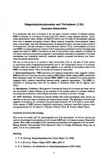
6

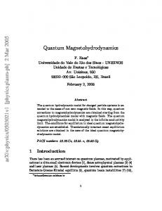
FIG. 1: Circularly-Polarized Alfv´en wave. B y component of the magnetic field for three different resolutions ∆x = {1/50, 1/100, 1/200}, together with the exact initial solution (black solid line). Clearly, the numerical solution provided by the resistive MHD implementation and the exact one overlap for a uniform conductivity σ = 106 and the highest resolution.

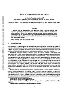
FIG. 2: Self-similar current sheet. B y component of the magnetic field at the initial t = 1 and final time t = 10. The exact solution at t = 1 is shown with a dashed blue line. The solution given by the analytic expression (47) at t = 10 (black solid line) is indistinguishable from the numerical solution obtained form the resistive MHD equations (red dashed line).

tial profile, it is convenient to apply periodic boundary conditions and compare the evolved profile after one full period with the initial one, in order to check the accuracy of our implementation. In particular, we consider a CP Alfv´en wave with a normalized amplitude ηA traveling along positive x-axis, in a uniform background magnetic field B0 with components

conductivity of σ = 106 , using the following resolutions: ∆x = {1/50, 1/100, 1/200}. In Fig. 1 we show the component B y at time t = 2, corresponding to one full period. By superimposing the results at t = 2 with the initial data at t = 0, it is evident that the numerical solution of the resistive MHD equations tends to the ideal-MHD exact solution for a high-enough conductivity and resolution. We have used both a linear reconstruction with monotonized-central (MC) slope limiter and the second order PPM reconstruction. The numerical solution converges to the exact one at second order when using PPM reconstruction and at second order with the linear reconstruction, exactly the same convergence rates than with the original ideal MHD system implemented in WhiskyMHD.

B i = {B0 , ηA B0 cos[k(x − vA t)], ηA B0 sin[k(x − vA t)]}. (44) For simplicity, we take v x = 0 and write the remaining velocity components as vy = −vA B y /B0 ,

vz = −vA B z /B0 ,

(45)

where  s  2 −1  2 2 2B 2η B A 0 0 2   . vA = 2 ) 1+ 1 − ρh + B 2 (1 + η 2 ) ρh + B02 (1 + ηA 0 A (46) By setting ρ = p = ηA = 1 and B0 = 1.1547, we fix the Alfv´en velocity to vA = 0.5. Therefore, in a computational domain centered at x = 0 with x ∈ [−0.5, 0.5], we expect the wave to return to its initial position after one full period t = L/vA = 2. The comparison of the numerical solution with the initial condition (44) at t = 0 gives us a measure of the error. In principle, the resistive MHD formalism would allow us to recover the ideal-MHD limit only for an infinite conductivity. In practice, however, the use of a conductivity as large as σ = 106 is sufficient to obtain a solution that converges to the ideal-MHD one with increasing resolution. As a result, we have chosen to perform simulations with a uniform

2. Self-similar Current Sheet

We next considera a test that involves the evolution of a selfsimilar current sheet, as proposed in Ref. [18]. This setup is useful for testing codes which solve the resistive MHD equations with a moderate conductivity regime, which we set to be σ = 100. In practice, the initial data consists in a magnetic field solely in the y-direction which changes sign in a thin current layer. Provided that the initial solution is in equilibrium (i.e., the pressure and density are constant, and the velocity is zero) and that the magnetic pressure is much smaller than the fluid pressure everywhere, then the evolution of the magnetic field is given by the simple diffusion equation ∂t B y − (1/σ) ∂x2 B y = 0, which will be responsible for the diffusive expansion of the current layer in response to the physical

7

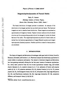
FIG. 3: Shock-tube Tests. B y component of the magnetic field at t = 0.4 for different resolutions ∆x = {1/100, 1/200, 1/400}. The highest resolution ∆x = 1/400 matches the exact ideal-MHD solution remarkably well.

resistivity (we are also assuming that E i = 0 = ∂t E i ). Under these simplified assumptions, the analytical solution of the diffusion equation is given, for t > 0, by  r  1 σ , (47) B y (x, t) = B0 Erf 2 ξ where ξ ≡ t/x2 and Erf is the error function. Clearly, as the evolution proceeds, the current layer expands in a self-similar fashion. Following [18, 19], we use as initial data the analytic solution (47) at t = 1 and set the density and pressure to be uniform with ρ = 1 and p = 50 respectively, while keeping the components of the electric field and velocity to zero initially. In our calculations we have used a computational domain with extents x = y = z ∈ [−5, 5] with a resolution of ∆x = 1/200. Furthermore, a linear reconstruction method was adopted with the further application of the MC limiter. In Fig. 2 we present the results we obtained by solving numerically the resistive MHD equations and the comparison with the exact solution (47) at t = 10 (black solid line). Clearly, the numerical solution (red dashed line) is indistinguishable from the analytic one, thus providing convincing evidence that the code can accurately describe resistive evolutions with intermediate values of the conductivity.

3. Shock-Tube Tests

We next consider the numerical solution of the standard of Brio and Wu shock-tube test [49] as adapted for its MHD implementation and using either a variety of uniform or spacedependent conductivities parameterized by the reference conductivity σ0 . More specifically, the left (L) and right (R)

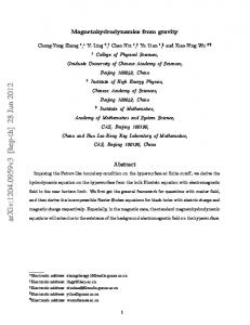
FIG. 4: Shock-tube Tests. B y component of the magnetic field for conductivities σ0 = {0, 10, 102 , 103 , 106 } at t = 0.4 and resolution ∆x = 1/200. For σ0 = 0 the magnetic field is governed by a wavelike equation, corresponding to the solution of the Maxwell equations in vacuum.

states are initially separated by a discontinuity at x = 0.5 and are given by [50] (ρL , pL , BLy ) = (1.0, 1.0, 0.5) , y (ρR , pR , BR ) = (0.125, 0.1, −0.5) , while all other variables are set to zero. The ideal-MHD evolution of the aforementioned setup with B x = 0 leads to two fast waves, one rarefaction propagating to the left and a shock propagating to the right of the discontinuity. The solution of this test in the ideal-MHD limit exists and is found in the exact ideal-MHD Riemann solver provided by Ref. [50]. For the rest of the one-dimensional tests, any comparison between the solution of the resistive MHD equations in the highconductivity regime and the exact solution of the ideal-MHD equations is performed with data obtained from the publicly available code [50]. All tests have been performed employing a linear reconstruction method with further application of the MC slope limiter. As a first setup of our shock-tube tests, we consider the case of a uniform high conductivity σ = σ0 = 106 and, in analogy with the Alfv´en-wave test in the high-conductivity regime, we verify that the solution of the coupled MaxwellHydrodynamics equations tends to the ideal-MHD exact solution [50] as the resolution is increased. Figure 3 reports the magnetic field component B y at t = 0.4 for the three resolutions ∆x = {1/100, 1/200, 1/400} considered. The high-resolution result matches the exact ideal-MHD solution so well that is difficult to distinguish them, thus providing the first evidence that our implementation is robust also in the presence of discontinuities. As a second setup of the shock-tube tests, we consider the case in which the conductivity is still uniform in space, but of different strength. In particular, we perform the same test

8

FIG. 5: Shock-tube Tests. The left panel shows the conductivity profile at t = 0.4 for non-uniform conductivity with different power laws, i.e., γ = {0, 6, 9, 12}. The γ = 0 case corresponds to the high-conductivity regime of the resistive MHD equations. The right panel reports instead the B y component of magnetic field for the same initial conditions as in the left one. The leftmost region tends to the ideal MHD solution, while the rightmost tends to the vacuum solution for γ = 12.

for σ = {0, 10, 102, 103 , 106 }, while keeping the resolution fixed at ∆x = 1/200. Figure 4 reports different solutions of the magnetic-field component B y given by the resistive MHD equations with different values of σ0 . It is important to note here that the solutions change smoothly from the ideal-MHD solution computed for σ0 = 106 , to the wave-like solution for σ0 = 0, which corresponds to the propagation of a discontinuity at the speed of light, corresponding to a solution of the vacuum Maxwell equations. The ability of treating the two extreme behaviours of the Maxwell-MHD equations via a resisitive treatment is an essential feature of our approach and a fundamental one in the description of the dynamics of magnetized binary neutron stars. As a final setup our of our suite of shock-tube test, we have considered the same initial data but now prescribed a nonuniform conductivity given by the expression σ = σ0 Dγ ,

(48)

where γ is an integer exponent we vary in the range γ ∈ [0, 12]. Thes prescription above introduces nonlinearities with respect to the conserved rest-mass density D and provides an intuitive way of tracking the dense fluid regions. It leads to low values of the conductivity in places were the plasma is tenuous and high values in more dense regions, which will prove very useful later on when evolving magnetized stars. However, this prescription is far from being realistic and normally a more general conductivity prescription σ = σ(D, τ, E) is to be seeked starting from micro-physical considerations. Following [19], we adopt the same initial data as before, however this time we change the exponent γ of Eq. (48) while maintaining the value of conductivity to σ0 = 106 . The results of this last test are reported in the left panel of Fig. 5, which show the profile of the conductivity at t = 0.4

for different values of the power-law exponent, i.e., γ = {0, 6, 9, 12}. Clearly, the conductivity follows the evolution of the rest-mass density, with a left-going rarefaction wave and right-going shock. It is interesting to note that our approach is able to track even very large variations in the conductivity, with jumps as large as eleven orders of magnitude across the computational domain. The right panel of Fig. 5, on the other hand, reports instead the magnetic field-component B y at t = 0.4 for the same initial conditions. As imposed by Eq. (48), the solution in the leftmost part of the computational domain, where the rest-mass density is very high, is controlled by a very high conductivity, which tends to σ0 = 106 . In turn, this implies that the solution for the magnetic field should approach the ideal-MHD limit in that region. On the other hand, in the rightmost region, where the rest-mass density is very low, the conductivity is correspondigly small and tending to zero for high values of γ. In such regions, therefore, the magnetic field is expected to behave as a wave, thus explaining the appearance of a moving peak for γ = 12. Overall, this suite of shock-tube tests, demonstrates that our numerical implementation is able to treat accurately both uniform and non-uniform conductivity profiles in one dimensional tests, independently of the steepness of the profiles and even in the presence of shocks.

B. Multidimensional Tests

We now focus on multidimensional tests that involve shocks in several directions, such as the two-dimensional cylindrical explosion and the three-dimensional spherical explosion test suggested in Ref.[1]. Despite the fact that there is no analytical solution for any of these tests, even in the ideal-MHD case, the symmetries of the problem can be of

9 -5

0

0.15

5

5 0.135

5

0

-5

0.05

5

5

5

0.12

0.03

0.105

0.02 0.01

0

y

y

0.09

0

0.075

-5

0 x

5

0

0

0

0.06

-0.01

0.045

-0.02

-5 0.03

-5

0.04

0.015

-5 -0.03

-5 0 x

-5

0

5

-0.04 -0.05

FIG. 6: Left Panel: Snapshot of the magnetic field component B x in the (x, y) plane at t = 4.0; Right Panel: Snapshot of the magnetic field component B y in the (x, y) plane at t = 4.0.

FIG. 7: Left Panel: One-dimensional cuts along the z-direction and at t = 4.0 of the the pressure. The black dashed line corresponds to the resistive code (the WhiskyRMHD code), while the blue dotted line corresponds to the ideal-MHD code, (the WhiskyMHD code). Right Panel: The same as in the left panel but for the Lorentz factor.

great help in verifying that the numerical implementation is correct and that it preserves the expected symmetries. Our approach in these tests will be therefore that of comparing the solution of the same multidimensional test as obtained with the ideal-MHD code presented in [11] and our new resistive WhiskyRMHD code in the limit of very high conductivities. The initial electric field is computed in such a way that it satisfies the ideal-MHD condition, i.e., E i = −ǫijk vj Bk , and all the tests have been performed adopting a linear reconstruction method and the minmod slope limiter.

1.

Cylindrical Blast-Wave

In the two-dimensional cylindrical blast-wave problem, we adopt a square domain with 200 grid cells per direction, in a range of (−6.0, 6.0) × (−6.0, 6.0). The setup of the problem consists of three regions. The innermost region with 0 ≤ r ≤ 0.8, for which the pressure and the density are set to p = 1, ρ = 0.01 respectively, the intermediate region which extends from 0.8 < r < 1.0 where r ≡ (x2 + y 2 )1/2 both the pressure and the density exponentially decrease, and the outermost region which is filled with an ambient plasma with p = 0.001, ρ = 0.001 and occupies the domain 1.0 ≤ r ≤ 6.0. The initial magnetic field is along the x-direction with an initial magnetic field strength of B0 = 0.05.

10 The numerical results are presented in Fig. 6, where we show that the magnetic field solution is regular everywhere and that there are no visible artifacts that could indicate a possible symmetry error in our implementation. Furthermore, when one-dimensional cuts of the resistive solution are plotted against the ideal-MHD solution obtained with the code presented in [11], the agreement is extremely good (this is not shown in Fig. 6).

2.

Spherical Blast-Wave

In the three-dimensional spherical blast-wave problem, the grid structure is similar, but the domain is now within the ranges (−6.0, 6.0) × (−6.0, 6.0) × (−6.0, 6.0). The problem setup consists of the same three regions as in the cylindrical blast wave problem, although here the radius r refers to the spherical-polar radial coordinate, and not to the cylindrical radius, i.e., r ≡ (x2 + y 2 + z 2 )1/2 . The corresponding solution of the spherical blast-wave problem in the (x, y) plane is essentially identical to the one already reported in Fig. 6 and for this reason we do not show it here. What we do show in Fig. 7, however, are onedimensional cuts along the z-direction of the pressure p and of the Lorentz factor W as computed with the ideal-MHD code (blue dotted line) and the resistive MHD code (black dashed line). This comparison, which is not expected to be exact given that the resistivity is large but not infinite, provides convincing evidence of the ability of our implementation to accurately describe higher-dimensional discontinuous flows in the high-conductivity regime.

magnitude smaller than the value of D at the center of the star. Furthermore, in the atmosphere we set the fluid velocity to zero and since σ = 0 there, the electric and magnetic fields are evolved via the Maxwell equations with zero currents (electrovacuum). This non-uniform conductivity prescription allows us to provide effective boundary conditions at the surface of the star for the exterior electrovacuum solution similar to those in Refs. [51, 52], but without the limitations of using an analytical solution for the interior of the star or the further complications of finding a suitable matching between the electromagnetic fields of the interior ideal-MHD solution and the exterior one. All the simulations reported hereafter have been performed adopting the PPM reconstruction scheme, for relativistic stars whose initial properties are summarized in Table II. 1.

Stable Star with confined magnetic fields

For the sake of simplicity, we consider as initial data spherical stars in equilibrium to which a poloidal magnetic field confined to the stellar interior is superimposed (see, e.g., [53– 55]). While the hydrodynamical quantities are consistent solutions of the Einstein equations, the magnetic field is added a-posteriori, with a consequent violation of the constraint at the initial time. In practice, however, this violation is always very small, even for the largest fields, and is quickly dominated by the violations introduced by the standard evolution. The toroidal vector potential that generates the poloidal interior magnetic field is expressed as [11] 2

Aφ = r2 max [Ab (P − Pcut ), 0] , C. Nonrotating Magnetized Stars

In the following Section we present the numerical results obtained from the evolution of nonrotating spherical stars in the presence of electromagnetic fields and for a variety of conductivities. In order to accurately model both the interior and the exterior of the star, we prescribe a spatial dependence of the electrical conductivity such that the ideal-MHD limit is recovered in the deep interior of the star (which is expected to be an excellent conductor) and such that the electrovacuum limit is recovered outside the star, where the density and the isotropic conductivity is expected to be negligibly small. This behaviour can be easily achieved assuming that the conductivity tracks the (conserved) rest-mass density, thus insuring a smooth transition between the two regimes. In practice, we have experimented with functional prescriptions of the type 2

σ = σ0 max [(1 − Datmo /D) , 0] ,

(49)

where σ ≃ σ0 is the conductivity in the regions of large restmass density (σ = σ0 at the stellar center) and σ = 0 in the atmosphere, where we set the conserved rest-mass density to its uniform value D = Datmo . In our calculations we normally set σ0 = 106 and Datmo to be about ten orders of

(50)

where Pcut is about 4% the central pressure Pc . The the star, initially computed with a polytropic EOS with Γ = 2, K = 100, has a gravitational mass M = 1.40M⊙ and is endowed with a poloidal magnetic field of strength Bc = 1012 G at the center of the star and β ≡ pmag /p = 4.49 × 10−13, with pmag the magnetic pressure. The magnetic field in the atmosphere is initially zero. For all of the evolutions presented hereafter we have used an ideal-fluid EOS with Γ = 2. We first examine the evolution of the magnetized star in the fixed spacetime of the initial solution (Cowlingapproximation). In the left panel of Fig. 8 we show with thin solid, dashed and dotted lines the evolution of the central restmass density normalized to its initial value ρc,0 in thin colored lines. The tests were performed using three spatial resolutions of ∆x = {0.4, 0.3, 0.2} km, corresponding respectively to N = {80, 120, 160} points across the finest AMR grid, which extends up to Rout = ±18 km. As customary in this type of tests, stellar oscillations are triggered by the truncation error and their amplitude decreases as the numerical resolution is increased. The importance of the test lays therefore in the calculation of the eigenfrequencies of the oscillations, which we find to be in very good agreement with those computed via perturbative analyses (not shown here) and with other hydrodynamics and ideal-MHD codes [11, 56]. In addition, a comparison with the ideal-MHD code [11] shows a very good

11 Star type MADM [M⊙ ] Mb [M⊙ ] Req [km] K Confined fields 1.40 1.51 12.00 100.0 Extended fields 1.33 1.37 32.56 372.0 Unstable model 2.75 2.89 16.30 364.7

Γ 2 2 2

Bc [G] # levels N 1012 4 80, 120, 160 2.4 × 1014 4 120 5 × 1015 5 272

Nstar Rout [km] 56, 80, 112 142 84 355 216 241

TABLE II: Properties of the magnetized star models used in the simulations. The columns report: the ADM and baryon masses in units of solar masses MADM and Mb respectively, the circumferential equatorial radius of the star in kilometers Req , the polytropic constant K, the polytropic index Γ, the value of the magnetic field in Gauss at the center of the star Bc , the number of refinement levels, the number of gridpoints on the finest level N , the number of gridpoints across the star Nstar for the different resolutions considered, the computational grid outer boundary in kilometers Rout .

FIG. 8: Left Panel: Evolution of the central rest-mass density of a nonrotating magnetized star for both the Cowling approximation (C; thin lines) and a dynamical spacetime (D; thick lines). Different line types mark different resolutions: dashed light blue ∆x = 0.4 km, dotted dark blue ∆x = 0.3 km, continuous black ∆x = 0.2 km. Middle Panel: The same as the left one but for the central magnetic field. Right Panel: The same as the middle one but different values of the conductivity σ0 . All lines refer to a resolution of ∆x = 0.2 km.

agreement in the evolution of the rest mass density, indicating that the oscillations are tracked correctly by our resistive MHD implementation. We next examine the same scenario, but in a fully dynamical spacetime and find also in this case a very good agreement with the ideal MHD solution. Still in the left panel of Fig.8 we report with thick solid, dashed and dotted lines the evolution of the central rest-mass central density in a dynamical spacetime for different resolutions. As well known from perturbation theory, the eigenfrequencies of oscillations are in this case lower but what is relevant to note is that the secular evolution in both the fixed and dynamical spacetimes are very similar, with variations in the central density that is less than a couple of percent over tens of dynamical timescales. The middle panel of Fig. 8 displays instead the evolution of the central value of the magnetic field, where lines of different color refer to different resolutions, while the thickness marks whether we are considering a fixed or a dynamical spacetime (thin for the Cowling approximation and thick for a full general-relativistic evolution). The corresponding power spectral density is shown in Fig. 9, where different line types refer to different resolutions and the dotted vertical lines mark the eigenfrequencies obtained from linear perturbation theory. The match between the numerical and perturbative results is clearly excellent and the differences in the fundamental mode

FIG. 9: Power spectral density of a full general-relativistic evolution of the central rest-mass density for a stable star with confined magnetic fields. Different line types refer to different resolutions. Shown with dotted vertical lines are the eigenfrequencies obtained from linear perturbation theory.

12 t = 0.000ms

t = 9.886ms

60

t = 18.590ms

60

60

logHΡL @grcm3 D

logHΡL @grcm3 D

14.80

13.30

20

12.80

20

40 x HkmL

60

13.80 13.30

20

12.80

12.30

12.30

11.80

11.80

0 0

14.80

40

14.30

z HkmL

z HkmL

13.80

0 0

14.80

40

14.30

20

40

12.47 11.30

20

x HkmL

10.13 8.97 7.80

0 0

60

13.63

z HkmL

40

logHΡL @grcm3 D

20

40

60

x HkmL

FIG. 10: Two-dimensional cuts on the (x, z) plane of the solution the rest-mass density (colorcode from white to red) and of the magnetic field lines and at times t = 0, 9.88, and 18.59 ms. The evolution refers to a nonrotating star in a dynamical spacetime. Note that although the magnetic field is contained in the star initially, it diffuses out as a result of numerical and physical resistivity.

at the highest resolution are . 0.5%. We note that, as for the central rest-mass density, the evolution of the central magnetic field is accompanied by a secular drift towards lower values, and this is simply the result of the intrisic numerical resistivity (we recall that these tests have been performed with the resistive code but for very large conductivities and hence in a virtual ideal-MHD regime). Clearly, the numerical resistivity decreases with resolution and this is exactly what the behaviour in the middle panel shows. It is interesting to note that while with sufficient resolution the resistive losses saturate to about 20% of the original magnetic field over ∼ 12 ms, these can be very large for low resolution and dissipate up to ∼ 85% of the initial magnetic field over the same time-span. These numerical resistive losses should be compared with the ones introduced instead by the physical resistivity and which can of course be much larger. This is shown in the right panel of Fig. 8, which is the same as the middle one, but where we have used the highest resolution (i.e., ∆x = 0.2 km) and varied the strength of the physical resistivity from σ0 = 106 to σ0 = 102 . Because the fluid velocities are essentially zero at this resolution, the magnetic-field evolution follows a simple diffusion equation with a Ohmic decay timescale which scales linearly with 1/σ. This is indeed what shown in the right panel of Fig. 8 where, after the initial transient, the solution settles to an exponential decay and where the magnetic field can be reduced of almost two orders of magnitude over 12 ms in the case of σ0 = 102 . Finally, we show in Fig. 10 two-dimensional cuts on the (x, z) plane of the rest-mass density (shown in a colorcode from white to red) and of the magnetic field lines for an oscillating star; the three panels refer to times t = 0, 9.88, and 18.59 ms, respectively. It is important to remark that although we start with a magnetic field that is initially confined inside the star, the inevitable presence of a small but finite numerical resistivity and our choice of a nonzero physical conductivity near the surface of the star [we recall that our conductivity follows the profile given in Eq. (49)], induce a slow but continuous “leakage” of the magnetic field, which leaves the star and fills the computational domain. Because the external magnetic field is essentially with a zero divergence and with a van-

ishingly small Laplacian (we recall that in the stellar exterior the resistivity is zero and the Maxwell equations tend to the those in vacuum), it is to a very good approximation a potential field, as shown by the clean dipolar-like structure. Clearly, the Ohmic diffusion timescale increases with resolution and therefore the relaxation of the magnetic field to a stationary dipolar-like structure takes place on longer timescales for the high-resolution simulation.

2.

Stable Star with extended magnetic fields

We next consider initial data for a spherical magnetized star with a poloidal magnetic field extending outside the star, as generated by the Magstar code from LORENE library [48]. The external magnetic field is dipolar and is computed by solving the Maxwell equations in vacuum, with boundary conditions given by the interior poloidal magnetic field. This solution is fully consistent with the Einstein equations and it provides accurate measurements of the stellar deformations in response to either rapid rotation or large magnetic fields [57]. More specifically, we have considered a nonrotating star modelled initially as polytrope with Γ = 2 and K = 372, having a gravitational mass M = 1.33 M⊙ , and endowed with a poloidal magnetic field of strength Bc = 5 × 1015 G. The magnetic field in the atmosphere is given by the electrovacuum solution, which has a dipolar structure. The evolutions have been carried out in a computational domain with outer boundary at Rout = 355 km and a resolution of ∆x = 0.7 km, corresponding to 60 points covering the positive part of finest grid which extends up to 44 km. Figure 11 displays in its left and middle panels twodimensional cuts on the (x, z) plane of the rest-mass density (shown in a colorcode from white to red) at the initial and final times, i.e., t = 0 ms and t = 37 ms. A rapid comparison among the three panels clearly shows the ability of the code to reproduce stably the evolution of this oscillating star also when the magnetic field extends in its exterior. The right panel of Figure 11, on the other hand, shows in its top part shows the evolution of the magnetic flux computed across a hemispheric

13 t = 0.000ms

t = 37.230ms

logHΡL @grcm3 D

240

logHΡL @grcm3 D

240

13.80

180

13.00 12.20

120

11.40

z HkmL

z HkmL

180

13.80 13.00 12.20

120

11.40

10.60

60

10.60

60 9.80

9.80

9.00

0 0

60

120 x HkmL

180

240

9.00

0 0

60

120 x HkmL

180

240

FIG. 11: Left and Middle Panels: Evolution of the magnetic field lines displayed at times t = 0 ms and t = 37 ms. The rest mass density is also shown with purple-red-yellow colors. Right Panel: The top part shows the evolution of the magnetic flux computed across a hemispheric surface at a radius r = 135 km, while the bottom part shows the power spectral density of the rest-mass density (black solid line) and of the magnetic flux (blue dotted line).

surface at a radius r = 135 km, which also shows signs of oscillations. We have computed the power spectrum of these oscillations and compared it with the corresponding one obtained for the central rest-mass density. The results of this comparison are shown in the bottom part of the right panel, with a black solid line referring to the rest-mass density a blue dotted line to the magnetic flux. The very good agreement between the two implies that the oscillations observed in the magnetic flux are essentially triggered by the oscillations in the rest-mass density.

3. Magnetized Collapse to a Black Hole

Our final and most comprehensive test is represented by the collapse to a BH of a magnetized nonrotating star. This is more than a purely numerical test as it simulates a process that is expected to take place in astrophysically realistic conditions, such as those accompanying the merger of a binary system of magnetized neutron stars [26, 27], or of an accreting magnetized neutron star. The interest in this process lays in that the collapse will not only be a strong source of gravitational waves, but also of electromagnetic radiation, that could be potentially detectable (either directly or as processed signal). The magnetized plasma and electromagnetic fields that surround the star, in fact, will react dynamically to the rapidly changing and strong gravitational fields of the collapsing star and respond by emitting electromagnetic radiation. Of course, no gravitational waves can be emitted in the case considered here of a nonrotating star, but we can nevertheless explore with unprecedented accuracy the electromagnetic emission and assess, in particular, the efficiency of the process and thus estimate how much of the available binding energy is actually radiated in electromagnetic waves. Our setup also allows us to investigate the dynamics of the electromagnetic fields once a BH is formed and hence to assess the validity of the no-hair theorem, which predicts the exponential decay of any electromagnetic field in terms of Quasi Normal Mode (QNM) emission from the BH.

Ours is not the first detailed investigation of this process and relevant previous studies are that in Ref. [51] and the more recent one in Ref. [52]. However, our approach differs from previous ones in that it correctly describes the gravitational dynamics of a collapsing fluid (the semianalytical work in Ref. [51], in fact, considered the more rapid collapse of a dust sphere, for which the Oppenheimer-Snyder (OS) analytic solution can be used [58]) and does not require any matching of the solution near the stellar surface (the fully relativistic work in Ref. [52] had to resort to an ingeniuous matching between the interior ideal-MHD solution and a force-free one in the magnetosphere), leaving the complete evolution of the electromagnetic fields to our prescription (49) of a nonuniform conductivity. Indeed, our solution is expected to be exactly the same as the force-free one except in regions where B 2 − E 2 < 0 and an anomalous resistivity appears. Since we can handle accurately such resistive regions, this test illustrates the capabilities of our resistive implementation and serves as a more realistic approach to this astrophysical scenario. In practice, we have considered the evolution of a nonrotating neutron star with a gravitational mass of 2.75M⊙ , which is chosen to sit on the unstable branch of the equilibrium configurations and is endowed with an initial poloidal magnetic field of strength Bc = 5 × 1014 G extending also in the exterior space. As for the previous stellar solutions, we use a polytropic EOS with Γ = 2 and K = 364.7 for the initial data and continue to use this isentropic EOS also for the subsequent evolution. The evolutions have been carried out in a computational domain with outer boundary at Rout = 241 km and a resolution of ∆x = 0.11 km, corresponding to 272 points covering the finest grid which extends up to ±15 km. Because the magnetic energy is only a small fraction of the binding energy, the hydrodynamical and spacetime evolution of the fluid star as it collapses to a BH is very similar to the unmagnetized case and this has been discussed in great detail in [59]. The most important difference, therefore, is in the dynamics of the magnetic field, and this is shown in Fig. 12, which reports two-dimensional cuts on the (x, z) plane of the

14 logH ΡL @grcm3D

t = 0.328 ms

120

logH ΡL @grcm3D

14.8

9.2

60

HSr L34 @ergscm2secD

1.6

30

0 0

90

0.0

-0.8

-0.8

0 0

-1.6

30

60 x HkmL

90

logH ΡL @grcm3D

14.8

10.6

9.2

9.2

60

HSr L34 @ergscm2secD

90

t = 1.091 ms

logH ΡL @grcm3D 14.8 13.4 12.0 10.6 9.2

60

HSr L34 @ergscm2secD 1.6

30

0.8

0.8

0.0

0.0

0.0

-0.8

-0.8

-0.8

-1.6

60 x HkmL

120

1.6

30

0.8

30

90

90

12.0

10.6

z HkmL

z HkmL

0 0

60 x HkmL

14.8

1.6

30

-1.6

30

120

13.4

90

12.0

HSr L34 @ergscm2secD

0 0

120

t = 0.987 ms

120

13.4

60

0.8

-0.8

logH ΡL @grcm3D

90

1.6

30

0.8 0.0

120

t = 0.656 ms

120

HSr L34 @ergscm2secD

0.0

-1.6

60 x HkmL

9.2

60

1.6

30

0.8

30

12.0 10.6

z HkmL

9.2

z HkmL

z HkmL

10.6

13.4

90

12.0

10.6

HSr L34 @ergscm2secD

14.8

13.4

90

12.0

60

logH ΡL @grcm3D

14.8

13.4

90

t = 0.568 ms

120

z HkmL

t = 0.000 ms

120

0 0

120

-1.6

30

60 x HkmL

90

0 0

120

-1.6

30

60 x HkmL

90

120

FIG. 12: Two-dimensional cuts on the (x, z) plane of the collapse to a BH of a magnetized NS. Shown with colors are the rest-mass density (colorcode from white to red) and the radial poynting vector (colorcode from blue to green) in units of 1034 , while thin lines reproduce the magnetic-field lines. The different snapshots refer to times t = 0, 0.32, 0.57, 0.65, 1.0 and 1.1 ms, and an apparent horizon is marked with a thin red line starting from t = 0.57 ms. Note that all the matter is accreted into the hole and that a quadrupolar QNM ringdown is clearly visible in the Poynting flux. logH ΡL @grcm3D

8

logH ΡL @grcm3D 14.8

14.8

13.4

13.4

12

12.0

12.0

10.6

10.6

10.6

9.2

9.2

0.8

8

HSr L34 @ergscm2secD

8 x HkmL

12

16

9.2

8

HSr L34 @ergscm2secD

1.6

4

0.8

1.6

4

0.8

0.0

0.0

0.0

-0.8

-0.8

-0.8

-1.6

4

12

12.0

1.6

0 0

logH ΡL @grcm3D

14.8

HSr L34 @ergscm2secD

4

t = 1.091 ms

16

13.4

z HkmL

z HkmL

12

t = 0.987 ms

16

z HkmL

t = 0.656 ms

16

-1.6

0 0

4

8 x HkmL

12

16

-1.6

0 0

4

8 x HkmL

12

16

FIG. 13: The same as the three bottom panels of Fig. 12 but with a linear scale of 15 km to highlight the dynamics near the horizon. It is now very clear that a closed set of magnetic field lines is built just outside the horizon at t = 1.0 ms, that is radiated away as QNM of the BH.

collapse to a BH of a magnetized NS. Shown with colors are the rest-mass density (colorcode from white to red) and the radial poynting vector (colorcode from blue to green), while thin solid lines reproduce the magnetic-field lines. At early times the star remains close to its initial state with the exception of a small transient induced by truncation error, which produces a small radiative outburst at t . 0.3 ms. As

the instability to gravitational collapse develops, there is a rearrangement of the external electromagnetic fields, driven by a toroidal electric field Eφ ≈ −vr Bθ produced in the interior of the perfectly conducting star, and which is continuous across the stellar surface. As the collapse proceeds, the restmass density in the center and the curvature of the spacetime increase until an appararent horizon is found at t = 0.57 ms

15 logH ΡL @grcm3D

t = 0.328 ms

120

logH ΡL @grcm3D

14.8

9.2

60

HB2-E 2L 23 @ergscm3D

0 0

30

-0.4

60 x HkmL

90

-0.8

-1.2

-1.2

0 0

120

t = 0.656 ms

120

logH ΡL @grcm3D

30

60 x HkmL

90

t = 0.987 ms

9.2

9.2

60

HB2-E 2L 23 @ergscm3D

30

60 x HkmL

90

120

120

t = 1.091 ms

logH ΡL @grcm3D 14.8 13.4 12.0 10.6 9.2

60

HB2-E 2L 23 @ergscm3D

0.0

30

-0.4

-0.8

-0.8

-1.2

-1.2

-1.6

90

90

12.0 10.6

z HkmL

z HkmL

0 0

60 x HkmL

14.8

10.6

-0.4

-1.6

30

120

13.4

0.0

30

-1.2

0 0

logH ΡL @grcm3D

90

12.0

HB2-E 2L 23 @ergscm3D

-0.4 -0.8

120

14.8

60

0.0

-1.6

120

13.4

90

HB2-E 2L 23 @ergscm3D

30

-0.4

-0.8

-1.6

30

9.2

60

0.0

0.0

30

12.0 10.6

z HkmL

9.2

z HkmL

z HkmL

10.6

13.4

90

12.0

10.6

HB2-E 2L 23 @ergscm3D

14.8

13.4

90

12.0

60

logH ΡL @grcm3D

14.8

13.4

90

t = 0.568 ms

120

z HkmL

t = 0.000 ms

120

0 0

-1.6

30

60 x HkmL

90

120

0.0

30

-0.4 -0.8 -1.2

0 0

-1.6

30

60 x HkmL

90

120

FIG. 14: The same as in Fig. 12, but where in addition to the rest-mass density (colorcode from white to red) and the magnetic-field lines (thin solid lines) we show the electrically-dominated regions (i.e. B 2 − E 2 < 0, colorcode from light blue to white in units of 1023 ).

and is marked with a thin red line in Fig. 12 (we have used the apparent-horizon finder described in [60]). As the stellar matter is accreted onto the BH (the rest-mass outside the horizon Mb, out = 0 is zero by t & 0.62 ms), the external magnetic field which was anchored on the stellar surface becomes disconnected, forming closed magneticfield loops which carry away the electromagnetic energy in the form of dipolar radiation. This process, which has been described through a simplified non-relativistic analytical model in Ref. [52], predicts the presence of regions where |E| > |B| as the toroidal electric field propagates outwards as a wave. This process can be observed very clearly in Fig. 13, which displays the same three bottom panels of Fig. 12 on a smaller scale of only 15 km to highlight the dynamics near the horizon. In particular, it is now very clear that a closed set of magnetic field lines is built just outside the horizon at t = 1.0 ms, that is radiated away. Note also that our choice of gauges (which are the same used in [61]) allows us to model without problems also the solution inside the apparent horizon. While the left panel of Fig. 13 shows that most of the rest-mass is dissipated away already by t = 0.65 ms (see discussion in [62] about why this happens), some of the matter remains on the grid near the singularity, anchoring there the magnetic field which slowly evolves as shown in the middle and right panels. A complementary view of the collapse process is also offered by Fig. 14, which reports, in addition to the rest-mass density (colorcode from white to red) and the magnetic-field

FIG. 15: Top Panel: Luminosity calculated at a distance r = 89 km from the compact object. The black dotted line represents the time at which the apparent horizon is formed and the black dashed line corresponds to the time at which all the matter is well within the horizon. Bottom Panel: Evolution of the total radiated energy normalized to the initial magnetic energy.

16

FIG. 16: Left Panel: QNM ringdown of the magnetic field as measured through the magnetic flux at r = 37 km. Again, the black dotted line represents the time at which the apparent horizon is formed and the black dashed line corresponds to the time at which all the matter is well within the horizon; the dot-dashed line represents instead our fit to an exponential decay. Right Panel: Logarithm of the absolute values of the magnetic and electric fluxes as normalized to the initial magnetic flux.

lines (thin solid lines), also the electrically-dominated regions (i.e. B 2 − E 2 < 0, colorcode from light blue to white). The larger scales used in this case makes it easier to follow the dynamics of the closed field lines that once produced near the horizon, propagate as dipolar radiation at infinity. The total electromagnetic luminosity Lrad emitted during the collapse and computed as surface integral of the Poynting flux over a spherical surface at 89 km is shown in the top panel of Fig. 15. Note the presence of a rise during the collapse and of several pulses after the stellar matter has been accreted onto the black hole. The vertical dotted line represents the time at which the apparent horizon is first found, while the vertical dashed line corresponds to the time at which all the matter is within the horizon (i.e. Mb, out = 0). The peaks in the electromagnetic luminosity correspond to the closed magnetic-field loops that disconnect from the star and trasport electromagnetic energy. The bottom panel of Fig. 15, on the other hand, reports the evolution of the total electromagnetic energy lost in radiation Erad and when normalized to the value of the initial magnetic energy outside the star, E0 . Our results indicate therefore a total electromagnetic efficiency which is ≃ 5%; this result is smaller than the estimate made in Ref. [51] (which was of ≃ 20%), but, besides the different initial data used, this difference can be easily accounted for by the fact that the gravitational collapse simulated here is considerably slower (and hence inefficient) than the OS one computed in [51], where matter is free falling. Our efficiency is also smaller than the one computed in Ref. [52] and which is ∼ 16% once the same definition for E0 is used. However, many other factors could be behind this difference, e.g., differences in the initial data (use of a dipole everywhere in contrast

to a dipole only outside the star as in our case), differences in the stellar models, differences in the numerical approach (treatment of the surface of the star of the transition between ideal and force-free MHD). A closer comparison between the two approaches will be carried out in a separate work. After BH formation, the luminosity decreases exponentially in a fashion which is typical of the QNM ringing of an electrovacuum electromagnetic field in a Schwarzschild BH spacetime. These QNMs are clearly visible also in the (absolute value of the) magnetic flux shown in the left panel of Fig. 16, from which a comparison with the perturbative expectations can be made. More specifically, by fitting the harmonic oscillations of the ringdown and the exponential decay we have computed the frequencies of the “ringing-down” magnetic-field flux for the l = 1 mode to be ω = 0.344054 − i 6.46731 kHz, corresponding to a nonrotating black hole of 2.74 M⊙. The agreement with the analytical value is excellent, with a relative error of only ∼ 0.7% for the real part of the frequency and ∼ 5.6% for the imaginary one [63]. Finally, as a measure of the accuracy of our simulation we can compare the magnetic flux with the corresponding electric flux, which should vanish in the continuum limit since no net electric charge should be present. This is indeed the case, as can be deduced from the right panel of Fig. 16, which reports the two fluxes normalized to the initial magnetic flux. Note that the electric flux is about 30 orders of magnitude smaller than the magnetic flux before BH formation, increasing after an apparent horizon is found, but remaining 15-10 orders of magnitude smaller.

17 V. CONCLUSIONS

We have introduced a general-relativistic resistive MHD formalism as an extension of the special relativistic resistive MHD formalism reported in Ref. [19] for a 3+1 decomposition of the spacetime. Our numerical implementation has been made within the Cactus computational infrastructure as a continuation of the already existing general-relativistic hydrodynamics code Whisky [56, 59] and of the ideal-MHD code WhiskyMHD [11]. Our numerical approach exploits Implicit-Explicit (IMEX) methods and allows us to treat astrophysical problems in which different spatial regions fall into different regimes of conductivities. The flexibility introduced by using the RungeKutta will allow us to consider not only more general Ohm laws and a variety of astrophysical dynamos [24, 64], but also to use better dispersion relations to calculate the velocities in the HLLE method and to describe more accurately nonrelativistic systems [65]. Our implementation has been tested for a number of stringent tests and its robustness has been verified. The specialrelativistic tests involved the propagation of circularly polarized Alfv´en waves, the evolution of current sheets and shocktubes in one dimension, cylindrical and spherical explosion tests in two and three dimensions respectively, the evolution of stable and the collapse of unstable magnetized stars in dynamical spacetime. We have compared our numerical results either with the analytical solution (in the cases where one exists), or with the numerical ideal-MHD solution (in the limit of high conductivity), proving that our implementation is suitable to describe regions with a wide range of conductivities, with or without large discontinuities and shocks. We have also considered genuinely general-relativistic tests in terms of the evolution of nonrotating magnetized stars either with fixed or fully dynamical spacetimes. Our stars have been endowed with magnetic fields of varying strength, either confined in their interior or permeating also the exterior space, and have been modelled with a non-uniform conductivity that allows us to recover the ideal-MHD limit in the interior of the star and such the electrovacuum limit outside the star. All of our results indicate that the resistive implementation is able to follow the evolution of the oscillations triggered by the small truncation errors and that the associated eigenfrequencies match well those either reported with other hydrodynamics and ideal-MHD codes [11, 66] or from perturbation theory.

[1] S. S. Komissarov, Mon. Not. R. Astron. Soc. 303, 343 (1999). [2] S. K. K. S. T. Kudoh, Astrophys. J 495, L63 (1998). [3] L. Del Zanna, N. Bucciantini, and P. Londrillo, Astron. Astrophys. 400, 397 (2003), arXiv:astro-ph/0210618. [4] C. F. Gammie, J. C. McKinney, and G. T´oth, Astrophys. J. 589, 458 (2003), astro-ph/0301509. [5] P. Anninos, P. C. Fragile, and J. D. Salmonson, Astrophys. J. 635, 723 (2005). [6] M. D. Duez, Y. T. Liu, S. L. Shapiro, and B. C. Stephens, Phys. Rev. D 72, 024028 (2005), astro-ph/0503420.

Finally, we have considered the challenging and comprehensive test represented by the gravitational collapse of a magnetized nonrotating star to a BH. This scenario has an astrophysical interest of its own as it could lead to the emission of electromagnetic radiation, potentially detectable. Indeed we have found that as the collapse proceeds, electrically dominated regions develop and lead to the development of magnetic-field loops that propagate at the speed of light, carrying away electromagnetic energy. Up to 5% of the initial magnetic energy can be lost in this way and the following evolution of the magnetic field follows a clean exponential decay, as expected by an electromagnetic perturbation in a Schwarzschild spacetime. The match of the measured QNMs and the perturbative predictions is well of a few percent or less. Our new code is now ready to be applied to study a variety of astrophysical scenarios. These include the modeling of the magnetosphere that could be produced after the merger of binary neutron stars, or when the hypermassive neutron star collapses to a BH and is surrounded by a hot torus. The work in Ref. [30] has already reported that under these conditions strong magnetic fields can be produced and that a jet-like magnetic structure can develop. It is exciting to consider whether the resistive losses that are expected in the process will provide sufficient energy to launch of a powerful jet, not yet observed in Ref. [30]. Also of great interest is to study BH magnetospheres and the origin of jets so as to answer the question of whether an ergosphere is critical for the development of the Blandford-Znajek mechanism. Finally, our approach is also well suited to study the properties of accretion disk onto BHs and to elucidate the role that resistive losses play on the whole energetic budget. We will report on these applications in forthcoming works.

Acknowledgments

This work was supported in part by the DFG grant SFB/Transregio 7; the computations were made at the AEI and also on the cluster RANGER at the Texas Advanced Computing Center (TACC) at The University of Texas at Austin through XSEDE grant No. TG-PHY110027. BG acknowledges support from NASA Grant No. NNX09AI75G and NSF Grant No. AST 1009396.

[7] M. Shibata and Y. Sekiguchi, Phys. Rev. D 72, 044014 (2005). [8] L. Ant´on, O. Zanotti, J. A. Miralles, J. M. Mart´ı, J. M. Ib´an˜ ez, J. A. Font, and J. A. Pons, Astrophys. J. 637, 296 (2006), astroph/0506063. [9] D. Neilsen, E. W. Hirschmann, and R. S. Millward, Classical Quantum Gravity 23, S505 (2006). [10] L. Del Zanna, O. Zanotti, N. Bucciantini, and P. Londrillo, Astron. Astrophys. 473, 11 (2007), 0704.3206. [11] B. Giacomazzo and L. Rezzolla, Classical Quantum Gravity 24, S235 (2007), gr-qc/0701109.

18 [12] B. D. Farris, T. K. Li, Y. T. Liu, and S. L. Shapiro, Phys. Rev. D 78, 024023 (2008), 0802.3210. [13] B. Zink, ArXiv e-prints (2011), 1102.5202. [14] D. Biskamp, Physics of Fluids 29, 1520 (1986). [15] E. N. Parker, Solar Physics 111, 297 (1987). [16] D. Giannios, D. A. Uzdensky, and M. C. Begelman, Mon. Not. R. Astron. Soc. 395, L29 (2009), 0901.1877. [17] M. Lyutikov, Mon. Not. R. Astron. Soc. 367, 1594 (2006), arXiv:astro-ph/0511711. [18] S. S. Komissarov, Mon. Not. R. Astron. Soc. 382, 995 (2007), 0708.0323. [19] C. Palenzuela, L. Lehner, O. Reula, and L. Rezzolla, Mon. Not. R. Astron. Soc. 394, 1727 (2009), 0810.1838. [20] M. Dumbser and O. Zanotti, Journal of Computational Physics 228, 6991 (2009), 0903.4832. [21] S. Zenitani, M. Hesse, and A. Klimas, Astrophysical Journal Lett. 716, L214 (2010), 1005.4485. [22] M. Takamoto and T. Inoue, Astrophys. J. 735, 113 (2011), 1105.5683. [23] O. Zanotti and M. Dumbser, Mon. Not. R. Astron. Soc. 418, 1004 (2011), 1103.5924. [24] N. Bucciantini and L. Del Zanna, ArXiv e-prints (2012), 1205.2951. [25] M. Anderson, E. W. Hirschmann, L. Lehner, S. L. Liebling, P. M. Motl, D. Neilsen, C. Palenzuela, and J. E. Tohline, Phys. Rev. Lett. 100, 191101 (2008), 0801.4387. [26] Y. T. Liu, S. L. Shapiro, Z. B. Etienne, and K. Taniguchi, Phys. Rev. D 78, 024012 (2008). [27] B. Giacomazzo, L. Rezzolla, and L. Baiotti, Mon. Not. R. Astron. Soc. 399, L164 (2009). [28] S. Chawla, M. Anderson, M. Besselman, L. Lehner, S. L. Liebling, P. M. Motl, and D. Neilsen, Phys. Rev. Lett. 105, 111101 (2010), 1006.2839. [29] B. Giacomazzo, L. Rezzolla, and L. Baiotti, Phys. Rev. D 83, 044014 (2011). [30] L. Rezzolla, B. Giacomazzo, L. Baiotti, J. Granot, C. Kouveliotou, and M. A. Aloy, Astrophys. J. 732, L6 (2011), 1101.4298. [31] Z. B. Etienne, Y. T. Liu, V. Paschalidis, and S. L. Shapiro, Phys. Rev. D 85, 064029 (2012), 1112.0568. [32] S. T. McWilliams and J. Levin, Astrophys. J. 742, 90 (2011), 1101.1969. [33] A. L. Piro, ArXiv e-prints (2012), 1205.6482. [34] D. Lai, ArXiv e-prints (2012), 1206.3723. [35] B. Paczynski, Astrophys. J. Lett. 308, L43 (1986). [36] D. Eichler, M. Livio, T. Piran, and D. N. Schramm, Nature 340, 126 (1989). [37] R. Narayan, B. Paczynski, and T. Piran, Astrophys. J. 395, L83 (1992). [38] F. Banyuls, J. A. Font, J. M. Ib´an˜ ez, J. M. Mart´ı, and J. A. Miralles, Astrophys. J. 476, 221 (1997). [39] A. Dedner, F. Kemm, D. Kr¨oner, C. D. Munz, T. Schnitzer, and M. Wesenberg, Journal of Computational Physics 175, 645 (2002). [40] D. Pollney, C. Reisswig, L. Rezzolla, B. Szil´agyi, M. Ansorg,

[41] [42] [43] [44] [45] [46] [47] [48] [49] [50] [51] [52] [53]

[54]

[55] [56]

[57] [58] [59]

[60] [61] [62] [63] [64] [65] [66]

B. Deris, P. Diener, E. N. Dorband, M. Koppitz, A. Nagar, et al., Phys. Rev. D 76, 124002 (2007). E. F. Toro, Riemann Solvers and Numerical Methods for Fluid Dynamics (Springer-Verlag, 1999). A. Harten, B. Engquist, S. Osher, and S. R. Chakrabarty, J. Comput. Phys. 71, 231 (1987). P. Colella and P. R. Woodward, J. Comput. Phys. 54, 174 (1984). A. Harten, P. D. Lax, and B. van Leer, SIAM Rev. 25, 35 (1983). http://www.cactuscode.org. E. Schnetter, S. H. Hawley, and I. Hawke, Classical Quantum Gravity 21, 1465 (2004). L. Pareschi and G. Russo, Journal of Scientific Computing 25, 129 (2005). http://www.lorene.obspm.fr. M. Brio and C. Wu, Journal of Computational Physics 75, 400 (1988), ISSN 0021-9991. B. Giacomazzo and L. Rezzolla, Journal of Fluid Mechanics 562, 223 (2006), gr-qc/0507102. T. W. Baumgarte and S. L. Shapiro, Astrophys. J. 585, 930 (2003), arXiv:astro-ph/0211339. L. Lehner, C. Palenzuela, S. L. Liebling, C. Thompson, and C. Hanna, ArXiv e-prints (2011), 1112.2622. M. D. Duez, Y. T. Liu, S. L. Shapiro, M. Shibata, and B. C. Stephens, Phys. Rev. Lett. 96, 031101 (2006), astroph/0510653. M. Shibata, M. D. Duez, Y. T. Liu, S. L. Shapiro, and B. C. Stephens, Phys. Rev. Lett. 96, 031102 (2006), astroph/0511142. M. D. Duez, Y. T. Liu, S. L. Shapiro, and M. Shibata, Phys. Rev. D 73, 104015 (2006), astro-ph/0605331. L. Baiotti, I. Hawke, P. Montero, and L. Rezzolla, in Computational Astrophysics in Italy: Methods and Tools, edited by R. Capuzzo-Dolcetta (MSAIt, Trieste, 2003), vol. 1, p. 210. M. Bocquet, S. Bonazzola, E. Gourgoulhon, and J. Novak, Astron. and Astrophys. 301, 757 (1995), arXiv:gr-qc/9503044. J. R. Oppenheimer and H. Snyder, Phys. Rev. D 56, 455 (1939). L. Baiotti, I. Hawke, P. J. Montero, F. L¨offler, L. Rezzolla, N. Stergioulas, J. A. Font, and E. Seidel, Phys. Rev. D 71, 024035 (2005). J. Thornburg, Classical Quantum Gravity 21, 743 (2004). L. Baiotti and L. Rezzolla, Phys. Rev. Lett. 97, 141101 (2006), gr-qc/0608113. M. Thierfelder, S. Bernuzzi, D. Hilditch, B. Bruegmann, and L. Rezzolla, Phys. Rev. D 83, 064022 (2010), 1012.3703. K. D. Kokkotas and B. G. Schmidt, Living Rev. Relativ. 2, 2 (1999), http://www.livingreviews.org/lrr-1999-2. A. Bonanno, L. Rezzolla, and V. Urpin, Astron. Astrophys. 410, L33 (2003), astro-ph/0309783. M. Takamoto and S.-I. Inutsuka, Journal of Computational Physics 230, 7002 (2011), 1106.1732. L. Baiotti et al., Phys. Rev. D 71, 024035 (2005), grqc/0403029.