b cand maximum a b c of the ratios give rational estimates of a b from below and from above. The case c = b gives the usual floor and ceiling functions.
GENERALIZATIONS OF THE FLOOR AND CEILING FUNCTIONS USING THE STERN-BROCOT TREE
GENERALIZATIONS OF THE FLOOR AND CEILING FUNCTIONS USING THE STERN-BROCOT TREE
Håkan Lennerstad, Lars Lundberg
Håkan Lennerstad, Lars Lundberg
Copyright © 2006 by individual authors. All rights reserved. Printed by Kaserntryckeriet AB, Karlskrona 2006.
ISSN 1101-1581 ISRN BTH-RES–02/06–SE
Blekinge Institute of Technology Research report No. 2006:02
Generalizations of the floor and ceiling functions using the Stern-Brocot tree Håkan Lennerstad, Lars Lundberg School of Engineering, Blekinge Institute of Technology, S-371 79 Karlskrona, Sweden {Hakan.Lennerstad, Lars.Lundberg}@bth.se Abstract We consider a fundamental number theoretic problem where practial applications abound. We decompose any rational number ab in c ratios as evenly as possible while maintaining � �the sum of numerators and the sum of denominators. The minimum ab c and maximum ab c of the ratios give rational estimates of ab from below and from above. The case c = b gives the usual � � floor and ceiling functions. We furthermore define the difference ab c , which is zero iff c ≤ GCD(a, b), quantifying the distance to relative primality. � �
� � A main tool for investigating the properties of ab c , ab c and ab c is the Stern-Brocot tree, where all positive rational numbers occur in lowest terms and in size order. We prove basic � �properties such that there is a unique decomposition that gives both ab c and ab c . It turns out that this decomposition contains at most three distinct ratios. The problem has arisen in a generalization of the 4/3−conjecture in computer science.
Keywords: Floor function, ceiling function, mediant, relative primality, Stern-Brocot tree.
1
Introduction
In this paper we study optimal ways to decompose a rational number ab in c ratios, while preserving the sum of numerators and the sum of denominators. This is done so that all ratios are as close as possible to ab . We are interested in the minimum, maximum of the ratios, and of the difference of these two numbers. The problem is a fundamental number theoretic problem, and has very practical implications. However, the problem has arisen in a computer science context. The main results in the present paper are important in the companion paper [7], which otherwise is independent. In that paper a general version of the 4/3-conjecture, well known in computer science, is solved.
1
The present paper is purely mathematical. Here we take advantage of the Stern-Brocot tree to prove the existence of optimal decompositions in c ratios, and to find these decompositions. Given three integers a, b andPc where 1 ≤ P c ≤ b, we consider sets of c quotients ab11 , ..., abcc so that a = c1 ai and b = c1 bi . Here all ai are integers and all bi are positive integers, i.e. 1 ≤ bi ≤ b for all i. Such a set is called a c-decomposition of ab . Pick a c-decomposition where min( ab11 , ..., abcc ) is maximal. ¥ ¦ ¥ ¦ For such a decomposition we denote ab c = min( ab11 , ..., abcc ). We call ab c the c¥ ¦ floor ratio of a and b. This term is motivated by the fact that we have ab 1 = ab ¥a¦ ¥a¦ and b b = b , so the quantity generalizes the floor function. We refrain from j k ¥ ¦ ¥ ¦ ¥ ¦ writing ab c with a fraction bar, as ab c , since da 6= ab c in general. db c We may similarly define a generalized ceiling function. § a ¨For a decomposition a1 ac a1 ac a1 ac , ..., where max( , ..., ) is minimal, we denote b1 bc b1 bc b c = max( b1 , ..., bc ), which is the c-ceiling ratio of a and b. We prove that there ¥ ¦is a decomposition fulfilling both the minimum and the maximum, i.e. where ab c = min( ab11 , ..., abcc ) § ¨ and ab c = max( ab11 , ..., abcc ) (Lemma 18). We furthermore define the ceiling-floor difference as lam jak hai = − . b c b c b c £ ¤ We have ab c = 0 if and only if c ≤ GCD(a, b), since only if c ≤ GCD(a, b) there are decompositions so that all ratios are equal. If a is not a multiple of b the £ ¤ difference ab c increases from 0 to 1 when c increases from 1 to b. The quantity £a¤ where c can be seen as a b c quantifies the distance to divisibility of a by b, h i £ ¤ crudeness parameter. This is reflected in the property da = ab dc/de (Lemma db c £ ¤ 11). The difference ab c has practical interpretations. One is the "unavoidable unfairness" if a objects are shared among b persons who are subdivided in c groups (see Section 4). The sequences of floor or ceiling ratios may be denoted without index, i.e. jak ³j a k jak ´ = , and , ..., l ab mb ´ l ab m ³l ab m1 . , ..., = b b b b 1 ¥ ¦ § ¨ ¥ ¦ The sequence ab §is ¨decreasing from ab to ab as a function of c, while ab is increasing from ab to ab . We here use the terms "increasing" and "decreasing" in the forms that allow equality — e.g. f (x) is increasing if f (x) ≤ f (y) for all x < y. The parameter c specifies the number of ratios in which to divide ab , slightly similarly to how the denominator b in ab specifies the number of parts in which to divide a. The notion of c as an "extra denominator" of a special kind is 2
a supported by that the abbreviation formula da db = b can be generalized to also include c, since we have ¹ º ∙ ¸ j a k » da ¼ lam hai da da = , = , and = db dc b c db dc b c db dc b c
for any positive integer d (Lemma 12). It is however more to the point to describe c as the degree of crudeness in how we estimate ab , alternatively to regard b − c + 1 as¥ the § ¨ of accuracy. This is natural since c = 1 give ¦ degree maximal accuracy, ab 1 = ab 1 = ab , while it is minimal for c = b where we get ¥ ¦ ¥ ¦ § ¨ § ¨ the floor and ceiling functions ab b = ab and ab 1 = ab . ¥ ¦ § ¨ In this paper we give basic properties of ab c and ab c and show how the cfloor and c-ceiling ratios effectively may be calculated by using the Stern-Brocot tree. The main reference for the Stern-Brocot tree is [4]. In this tree all positive rational numbers are generated exactly once, and all occur in shortest terms. The link between the c-floor and c-ceiling ratios and the Stern-Brocot tree is provided by the operation a1 a2 a1 + a2 ⊕ = , b1 b2 b1 + b2 a1 a2 2 here denoted by ⊕. The number ab11 +a +b2 is called the mediant of b1 and b2 . It is the main operation of construction of the Stern-Brocot tree, and expresses that the sums of numerators and denominators are preserved in a decomposition. In Section 4 applications in number theory and discrete linear algebra are described briefly. The operation ⊕ has natural practical applications. Consider a situation where we have a1 kg of a certain gas in a container of volume b1 litres, with density a1 /b1 , and similarly for a2 kg of a certain gas in a neighbouring container of volume b2 litres. If the containers are merged, for example by removing a wall between the containers, we get the density (a1 + a2 )/(b2 + b2 ) in the larger merged volume. This instance has obvious discrete counterparts if a1 , a2 , b2 and b2 are all integers. In this paper we are interested in the inverse mediant operation, meaning that we will go backwards in the Stern-Brocot tree. Given two numbers a and b, we want to find a decomposition with ab11 ⊕ ... ⊕ abcc = ab . We are interested in a decomposition that is uniform, i.e., the ratios ab11 , ..., abcc should be as equal as possible. This problem is trivial for continous sets of numbers, in which case all ratios can be taken to £ be § ¨ It is ¥ not ¤ equal. ¦ trivial if ai ∈ Z and bi ∈ Z+ for all i, and the difference ab c = ab c − ab c quantifies the distance to an even distribution. For discrete sets we thus define:
Definition 1 Assume that a ∈ Z and b ∈ Z+ . A decomposition ab = ab11 ⊕ ... ⊕ abcc is uniform from below if there is no other decomposition with larger min( ab11 , ..., abcc ). Similarly, it is uniform from above if there is no other decomposition with smaller max( ab11 , ..., abcc ). It is uniform if it has both properties.
3
It turns out that for any ab there exist a uniform partition. Furthermore it is unique and contains at most three distinct ratios (Lemma 18). The § ¨SternBrocot tree also provides a fast algorithm to calculate the numbers ab c and ¥a¦ b c.
The paper is organized as follows. In Section 2 we present basic properties of the mediant and of the Stern-Brocot tree, concluding with previous research. In Section 3 we present and prove basic properties of the c-floor and the c-ceiling ratios, and the ceiling-floor difference. In Section 4 a few applications of these functions are discussed.
2 2.1 2.1.1
The mediant and the Stern-Brocot tree Previous research Number theory and the Stern-Brocot graph
Moritz Abraham Stern (1807—1894) succeeded Carl Friedrich Gauss in Göttingen. In 1858 he published the article Über eine zahlentheoretische Funktion [8], which contains the first publication of a tree which later came to be known as the Stern-Brocot tree. Independently, the clockmaker Achille Brocot 1861 presented the same tree in a paper about efficient use of systems of cogwheels [2]. Thus, from the very beginning the number theoretic content of the tree was accompagnied by applications, similarly to how this paper has emerged from problems in the computer science companion paper [7] (see Section 4). The Stern-Brocot tree was reintroduced by R. Graham, D. Knuth and O. Patasnik in [4], and has since then been the subject of research. For example, in [6] M. Niqui devises algoritms for exact algorithms for rational and real numbers based on the Stern-Brocot tree. 2.1.2
Computer science
Computer science problems are often very close to pure combinatorial or number theoretic problems. In a well-known binpacking problem we have n positive numbers x = (x1 , ..., xn ) and want to find a partitionPA of these numbers in k sets A1 , ..., Ak , k < n, so that f (A, x) = max1≤j≤k ( i∈Aj xi ) is minimal. We may denote this minimum by fe(x) = minA f (A, x) In the 4/3-conjecture two cases of binpacking are compared in the case k = 2. Normal binpacking, as above, is compared to a counterpart with an extra liberty during the packing. Here one of the numbers xi may be split in two positive numbers xi,1 and xi,2 whose sum is xi . We denote by f 0 (A, x) = P minsplit a xi (max1≤j≤k ( i∈Aj xi )) and fe0 (x) = minA f 0 (A, x). It is trivial that minx (f /f 0 ) = 1. The 4/3-conjecture states that maxx (f /f 0 ) = 4/3. This statement was conjectured by Liu 1972 [5] and proved by Coffman and Garey 1993 [3], all in a computer science context.
4
In computer science context, a set of numbers (x1 , ..., xn ) may represent a parallel program, the k partition sets correspond to the processors of a multiprocessor with k processors, a partition A is a schedule of the parallel program, and a split of a program from xi into xi,1 and xi,2 , where xi = xi,1 + xi,2 , is called a preemption. A partition where splits are allowed is then called a preemptive schedule. Braun and Schmidt proved 2003 a formula that compares preemptive schedules with i preemptions to a schedule with unlimited number of preemptions in the worst case, using a multiprocessor with m processors [1]. The comparison is made in terms of the ratio of completion times for a program that maximizes this ratio, when assuming optimal schedules in both cases. They show that no more than m − 1 preemptions are needed in the unlimited case. They generalized the bound 4/3 to the formula 2 − 2/(m/(i + 1) + 1), which also may be written as 2m/(m + i + 1). The paper [7] generalizes the problem considered by Braun and Schmidt into an optimal comparison of i preemptions to j preemptions, using a multiprocessor with m processors. In the case j ≤ m − i − 1 we find the optimal bound 2
bj/(i + 1)c + 1 . bj/(i + 1)c + 2
It turns outj that ink the case j ≤ m − i − 1, the floor ratio provides an explicit i+j+1 . This problem was a source for the present formula: 2 2i+j+2 min(m,i+j+1)−j paper.
2.2
The mediant — basic properties
2 In this section we consider properties of the mediant operation ab11 ⊕ ab22 = ab11 +a +b2 . First we formulate immediate properties. a2 a1 a2 a1 a2 2 It is obvious that ab11 < ab11 +a +b2 < b2 if b1 < b2 , unless b1 = b2 , in which case a1 a1 +a2 a2 b1 = b1 +b2 = b2 . The strict inequalities are important for the Stern-Brocot tree. The mediant operation is associative, ( ab11 ⊕ ab22 ) ⊕ ab33 = ab11 ⊕ ( ab22 ⊕ ab33 ), so we may simply write ab11 ⊕ ab22 ⊕ ab33 , and commutative ab11 ⊕ ab22 = ab22 ⊕ ab11 . We will 1 2 c also need the rule a1 +db ⊕ a2 +db ⊕ ... ⊕ ac +db = ab11 ⊕ ab22 ... ⊕ abcc + d. We assign b1 b2 b a1 a2c higher priority to ⊕ than +, so that b1 ⊕ b2 + d is to be read ( ab11 ⊕ ab22 ) + d. The mediant can be regarded as a weighted mean value. The quantity w1 x1 + w2 x2 is the arithmetic weighted mean value of the two numbers x1 and x2 , where the sum of the weights w1 and w2 is required to be one: w1 + w2 = 1. a c The mediant a+c b+d of b and d can be thought of as a weighted mean value, as
a+c b a d c = + , b+d b+d b b+dd b d and w2 = b+d are determined by the denominators i.e, the weights w1 = b+d only. We have similarly for n numbers
a1 a1 an an b1 bn ⊕ ... ⊕ = + ... + . b1 bn b1 + ... + bn b1 b1 + ... + bn bn 5
We will use this mean value property in Section 3 (Lemma 17). Of course, when considering weighted mean values, the weights w1 , ..., wn are usually considered to be independent of x1 , ..., xn . The above remark has a significance as a way of a c more exactly specify where a+c b+d is positioned relatively to b and d . Note also that this mean value is not a well-defined mean value of rational numbers, since da1 a2 a1 a2 db1 ⊕ b2 6= b1 ⊕ b2 in general. It is rather a mean value of pairs of numbers. 2 We remark that the mediant operation ab11 ⊕ ab22 = ab11 +a +b2 is isomorfic to the vector addition in linear algebra: (a1 , a2 ) + (b1 , b2 ) = (a1 + b1 , a2 + b2 ). This connection is further discussed in Section 4.2.
2.3 2.3.1
The Stern-Brocot tree Stern-Brocot sequences
The Stern-Brocot tree is generated by starting with the sequence 01 , 10 . Iteratively, longer sequences are generated by inserting mediants in all intermediate spaces. Hence, the first Stern-Brocot sequences are S0 S1 S2 S3 S4
0 1 = ( , ) 1 0 0 1 1 = ( , , ) 1 1 0 0 1 1 2 1 = ( , , , , ) 1 2 1 1 0 0 1 1 2 1 3 2 3 1 = ( , , , , , , , , ) 1 3 2 3 1 2 1 1 0 0 1 1 2 1 3 2 3 1 4 3 5 2 5 3 4 1 = ( , , , , , , , , , , , , , , , , ). 1 4 3 5 2 5 3 4 1 3 2 3 1 2 1 1 0
The following figure shows the common way to depict Stern-Brocot tree in the literature, here including up to the fifth generation.
6
Fig. 1 The Stern-Brocot tree - S5 . Since the mediant is a weighted mean value, the numbers are distinct, and all sequences Sn are in increasing order. 2.3.2
Generations
If we omit numbers that are already generated, we can talk about generations of numbers, which will be important in this paper. The first generations are then the following: G0 G1 G2 G3 G4
0 1 = ( , ) 1 0 1 = ( ) 1 1 2 = ( , ) 2 1 1 2 3 3 = ( , , , ) 3 3 2 1 1 2 3 3 4 5 5 4 = ( , , , , , , , ). 4 5 5 4 3 3 2 1
Clearly, Sn = ∪ni=0 Gi and Gn = Sn \Sn−1 . We denote the generation number of a ratio ab by g( ab ), i.e. ab ∈ Gg( ab ) . Each positive rational number has a unique generation number, this follows from that each rational number occur exactly once in the tree (Theorem 2). It is obvious that |Gn | = 2n−1 except that |G0 | = 2, and that |Sn | = 2n + 1. Each number is a mediant of two numbers. These two numbers may by the terminology of graph theory be called parents. Since every second number in a 7
Stern-Brocot sequence is generated in the last step, and all other numbers in earlier steps, each number has one parent that belong to the previous generation and another that belongs to an earlier generation. The number 11 is the only exception to this. We call a parent in the previous generation the close parent, and the other parent the distant parent. 2.3.3
The tree and the graph
When depicting the Stern-Brocot tree in the literature, it is a tradition to denote the tree in a simplified and somewhat incorrect way. Edges to close parents are represented only. When disregarding the other edges, the Stern-Brocot tree is a binary tree, exept for the generation consisting of 01 and 10 . When taking both kinds of edges into account, the graph is not a tree, if it is regarded as an undirected graph. For the results in this paper we need both kinds of edges. In the following figure the distant parent-offspring edges are marked with a dotted line.
Fig 2 The Stern-Brocot graph up to fifth generation — S5 = ∪5i=0 Gi . When we expicitely need both kinds of edges, we will talk about the SternBrocot graph. We then regard the graph as a directed graph where the edges are directed from lower to higher generations. As a directed graph it is a tree since there are no cycles. We use the term Stern-Brocot graph to emphasize that both kinds of egdes are equally important. In the following argument, we exempt the nodes 01 and 10 . Considering close edges only, each node has one parent and two offsprings. Considering all edges, each node has two parents and an infinite number of offsprings, two in each higher generation. The graph is infinitely large, alternatively sufficiently large.
8
We furthermore remark that the size order among the entries from left to right is always preserved. Geometrically this means that the graph is a planar graph — the branches do not cross. The branches do not even shadow each other if we imagine the sun above the tree positioned in zenit. 2.3.4
Stern-Brocot pairs
Nodes that are co-parents, i.e. has a common offspring, play an important role in this paper. A pair of rational numbers that are parents to ab is called the Stern-Brocot pair of ab , and is denoted by SB( ab ). By the construction, each ratio ab has a unique pair of parents. Note that ( ab11 , ab22 ) = SB( ab ) implies a1 a2 a 2 3 b1 ⊕ b2 = b , but the converse implication is usually false. For example, ( 5 , 7 ) 5 1 4 1 4 5 is the Stern-Brocot pair of 12 , but ( 5 , 7 ) is not, although 5 ⊕ 7 = 12 . We write the pair in size order, so if ( ab11 , ab22 ) is a Stern-Brocot pair we know that ab11 < ab22 . The significance of Stern-Brocot pairs is that it provides a decomposition where the numbers are as close as possible to the decomposed number. Note that if ( ab11 , ab22 ) is a Stern-Brocot pair there are no ratios in lowest terms in the interval ( ab11 , ab22 ) that have denominator smaller than b1 + b2 . Except for the Stern-Brocot pair ( 01 , 10 ), the two members of a Stern-Brocot pair always belong to different generations. Each Stern-Brocot pair ( ab11 , ab22 ) defines an infinite branch in the tree by repeated mediant-addition of the element that belongs to the lower generation. If g( ab11 ) > g( ab22 ) the branch runs to the right immediately below the element ab22 : BR (
a2 a1 + na2 )={ , n = 0, 1, 2, ...}, b2 b1 + nb2
while if g( ab11 ) < g( ab22 ) it goes to the left below the ratio BL (
a1 b1 :
a1 na1 + a2 )={ , n = 0, 1, 2, ...}, b1 nb1 + b2
Note that BR ( ab22 ) goes to the right but appears to the left of ab22 , and analogously for BL (see Fig 3). For example, the first two branches in the tree are BL ( 01 ) and BL ( 10 ), where BL ( 01 ) consist of all ratios where the numerator is 1, { n1 , n ∈ N}, while BR ( 10 ) is the set of natural numbers N ={1, 2, 3, ...}. The next two n branches are BR ( 11 ) = { n+1 , n ∈ N} and BL ( 11 ) = { n+1 n , n ∈ N}. Let us consider a certain node in the tree as a distant parent. Then all close co-parents to that node are located in the two branches below. Thus, the set of all co-parents to ab in higher generations is C( ab ) = BL ( ab ) ∪ BR ( ab ). Of course, the two branches never intersect.
9
Fig 3 Branches BL ( 12 ) and BR ( 12 ) below 12 .
2.3.5
Anchestor sequences
We use the term ancestor sequence A( ab ) to a ratio ab for the sequence containing all parents, parent’s parents, and so on, in size order. The ratio itself is included in the anchestor sequence. We only include one of the anchestors 01 and 10 . If a 0 1 b ≤ 1 the anchestor 1 is included, otherwise 0 is included. It follows from the construction that the anchestor sequence contains exactly one member for each generation from 0 to g( ab ). The anchestor sequence A( ab ) is a subsequence to S(g( ab )), and forms a conelike set in the Stern-Brocot tree. For example, the anchestor sequence of 25 is A( 25 ) = ( 01 , 13 , 25 , 12 , 11 ).
10
Fig 4 A( 58 ) — anchestor set of
5 8
inside double lines.
a that occur in the As we §shall ¨ see,¥ the ¦ numbers in A( b ) are the numbers a a sequences b and b . The floor sequence consists of ab and the numbers in A( ab ) to the left of ab , while the ceiling sequence consists of ab and those to the right. In Section 3 we prove this and specify exacly how c is related to the members in the set A( ab ). We sometimes use the term anchestor set, instead of anchestor sequence, if the order is irrelevant
2.3.6
Proofs of basic properties of the Stern-Brocot tree
We next establish fundamental properties of the Stern-Brocot tree. The proofs follow those in [4]. Theorem 2 Each non-negative rational number occurs exactly once in the SternBrocot tree, and in lowest terms. Proof : No number can occur twice or more, since a second occurence in a Stern-Brocot sequence would violate the strict increasing order of numbers. We next show that all numbers in the tree are in lowest terms. Of course, the ratio Ll is in lowest terms if there are integers a and b so that la + Lb = 1. We show by induction that we have Lr − lR = 1 if Ll , Rr are adjacent numbers r are in in any Stern-Brocot sequence. From this it follows that both Ll and R lowest terms.
11
It is clear that the pair 01 , 10 fulfil the condition Lr−lR = 1. For the induction it is enough to show that if we have Lr − lR = 1, then L(l + r) − l(L + R) = 1 is also true. This is a trivial calculation. Finally we prove that any ratio ab ≥ 0, where a and b are relatively prime, appears in the Stern-Brocot tree. For this we use the natural binary search algorithm in the tree, starting with ( 01 , 10 ), where we in each step pick the interval l+r l+r r l+r ) or ( L+R ,R ) that contains ab . A third possibility is L+R = ab , in which ( Ll , L+R a case we have found the appearence of b in the tree. We need to show that this third case necessarily happens at some point during the search algorithm. r We will show that from the inequalities Ll < ab < R and Lr − lR = 1 it follows that l + L + r + R ≤ a + b. Since at least one of the numbers l, L, r and R increase by at least one in each step of the iteration, while a and b are r constants, the inequalities Ll < ab < R cannot be valid for an infinite number of l+r a steps. Hence, the third case L+R = b necessarily happens. In proving l + L + r + R ≤ a + b, we start by noting that the inequalities l a r < L b < R give aL − bl ≥ 1 and br − aR ≥ 1. If these inequalities are multiplied by r + R respective l + L we get (aL − bl)(r + R) ≥ r + R, (br − aR)(l + L) ≥ l + L. Addition of the inequalities and cancellation to the left gives a(Lr − Rl) + b(−lr + rL) ≥ l + L + r + R, so from Lr − lR = 1 we get a + b ≥ l + L + r + R. The theorem is proved. In order to describe how rapidly the ratios grows in the tree, it is well known that the denominators of the numbers x ∈ Gn , x < 1 are at least n and at most Fn . Here Fn is the n:th member in the Fibonacci sequence 1, 1, 2, 3, 5, 8, 13, ..., defined iteratively by Fn+2 = Fn+1 + Fn and F0 = 1, F1 = 1. Furthermore, the Stern-Brocot tree gives the best possible rational approximations of an irrational number. We may extend the definition of an anchestor set to an irrational number q, by iteratively picking an interval ( ab11 , ab22 ) to which q belongs as in the proofs of Theorem 2, giving an infinite anchestor set A(q). The set contains the best rational approximations of q with limited denominator: Theorem 3 Suppose that q > 0 is irrational. If ab ∈ / A(q) and q < ab , then c c a there is a ratio d ∈ A(q) so that d ≤ b and q < d < b . Similarly, if ab ∈ / A(q) and q > ab , then there is a ratio dc ∈ A(q) so that a c d ≤ b and b < d < q. 12
For a proof, see [4]. √ For example, the anchestor set of the golden mean φ = ( 5 + 1)/2 ≈ 1.61803... is A(φ) = { 10 } ∪ {Fn /Fn−1 , n ∈ N}. Thus, ratios of Fibonacci numbers give best possible rational approximations of φ. We √ remark that Fn can explicitly be calculated using φ as Fn = (φn − (−φ)−n / 5. We conclude this section by contributing to the knowledge about the SternBrocot graph with a graph theoretic observation. We here study the SternBrocot graph and not the tree — both kinds of edges are important. This graph is a directed graph where each edge has a direction from a parent to its offspring. n−1 an k−1 A path from ab00 to abnn is a sequence of nodes ( ab00 , ab11 , ab22 , ..., abn−1 , bn ), where abk−1 ak is a parent to bk for all k = 1, ..., n. The observation says that the number of paths from a ratio to the closest first anchestor, 01 or 10 , simply is given by the denominator of the ratio. Theorem 4 For a ratio ab ≤ 1, the number of distinct paths in the Stern-Brocot graph from 01 to ab is b. For a ratio ab > 1, the number of distinct paths from 10 to ab is b. Proof : We prove this by induction.Suppose that ab ≤ 1. The induction starts with the observations that 11 has denominator 1 and one single path to 01 , which takes care of the case ab = 1, and that 12 has denominator 2 and two paths to 01 . For 12 , there is one path directly from 01 , the path ( 01 , 12 ) and one via 11 , which is the path ( 01 , 11 , 12 ). For ab < 1, let ab00 be the close parent and ab11 the distant parent. Thus, a0 +a1 a0 a1 a 0 b = b0 +b1 . By the induction hypothesis, b0 has b0 paths to 1 and b1 has b1 0 paths to 1 . Now, any path from ab to 01 goes first to the close parent ab00 or to the distant parent ab11 . If the distant parent ab11 is the first node, ab00 do not belong to the path. Hence, the set of paths starting with ab00 is disjoint to the set of paths starting with ab11 . It follows that the total number of paths from ab to 01 is b0 +b1 . Since this is the denominator of ab , the theorem is proven for ab ≤ 1. The proof in the case ab > 1 is very similar.
3
Main results
3.1
Fundamental properties of
¥a¦
b c
We start by proving that for fixed a and b, increasing as functions of c.
and
¥a¦
b c
§a¨
b c
is decreasing and
§a¨
b c
is
Lemma ¥a¦ ¥ a5¦ For fixed§ aa¨ and§b, ¨we have for all c = 1, ..., b − 1 the inequalities a ≥ and ≤ b c b c+1 b c b c. Proof : We prove
¥a¦
b c
≥
¥a¦
b c+1 .
13
For any (c+1)-decomposition has the property
ac+1 bc+1
min(
a1 ac ac+1 b1 , ..., bc , bc+1 ,
the c-decomposition
a1 ac b1 , ..., bc ⊕
ac ac+1 a1 ac ac+1 a1 , ..., ⊕ ) ≥ min( , ..., , ), b1 bc bc+1 b1 bc bc+1
c+1 c+1 since min( abcc , abc+1 ) ≤ abcc ⊕ abc+1 . Perhaps it is possible to find other c-decompositions that increase the left side even more. Thus, for an optimal (c+1)-decomposition a1 ac ac+1 b1 , ..., bc , bc+1 , we have
jak a1 ac ac+1 a1 ac ac+1 , ..., ⊕ ) ≥ min( , ..., , )= . b c+1 b c b1 bc bc+1 b1 bc bc+1 § ¨ By an analogus argument for ab c , the lemma is proved. jak
≥ min(
We next consider the two cases of ratios ab that are not represented in the Stern-Brocot tree: negative ratios and ratios which are not in lowest terms. 3.1.1
Positive numerators are enough
By the next lemma it is enough to consider a = 0, ..., b − 1. Lemma 6 For all a ∈ Z and b ∈ Z+ , we have ¹ º jak a a mod b = b c+ , b c b b c » ¼ lam a a mod b = b c+ , and b c b b c ∙ ¸ hai a mod b = b c b c Proof : Consider a decomposition ab11 , ..., abcc . If we insert ai = b ab cbi + ri , i = 1, ..., c, into the minimum min( ab11 , ..., abcc ), we obtain min(
b a cb1 + r1 b a cbc + rc ac a1 , ..., ) = min( b , ..., b ) b1 bc b1 bc a rc r1 = b c + min( , ..., ). b b1 bc
By summing the relations ai = b ab cbi + ri , i = 1, ..., c, it also follows that c X
ri = a mod b.
i=1
Thus, for each decomposition ab11 , ..., abcc , there is a decomposition rb11 , ..., rbcc with Pc a1 ac r1 rc a i=1 ri = a mod b and where min( b1 , ..., bc ) = b b c + min( b1 , ..., bc ). The two first equalitites follow by maximizing or minimizing among the decompositions. 14
The third equality
hai b
c
∙
¸
a mod b = b
c
follows immediately from the first two equalities and lemma is proven.
£a¤
b c
=
§a¨
b c
−
¥a¦
b c
. The
This lemma seems to unravel a certain asymmetry between the floor and ceiling functions, since the floor function b ab c occurs in both the floor and ceiling ratio statements. This is however superficial, § and ¨ follows from the preference to use positive numbers if possible. Perhaps ab c = d ab e + d a modb b−b ec is a more ¥ ¦ b cc . appropriate counterpart to ab c = b ab c + b a mod b
£ ¤ In fact, the difference ab c has an extra symmetry, from which if follows that only at most db/2e values of a give distinct values. Lemma 7 For all a ∈ Z and b ∈ Z+ , we have ∙ ¸ ∙ ¸ hai b−a −a = = . b b b c c
§ ¨ ¥ ¦ is an optimal decomposition for ab c and ab c ³ ³ ´ ´ written in decreasing order, so that max ab11 , ..., abcc = ab11 and min ab11 , ..., abcc = ³ ³ ´ ´ ac a1 ac = − abcc and min − ab11 , ..., − abcc = − ab11 , so bc . Then max − b1 , ..., − bc Proof : Suppose that
a1 ac b1 , ..., bc
¹
º −a b c » ¼ −a b c
Hence,
and the lemma follows from
hai
b £ −a ¤ b
c
c
=
= −
lam
= −
b
∙
−a = b h i b−a b
b c jak ¸
c
.
c
,
c
, by Lemma 6.
It is furthermore enough to consider decompositions whith ratios in the closed interval (b ab c, d ab e). ³ ´ Lemma 8 There is a decomposition ab11 , ..., abcc where abii ∈ [b ab c, d ab e] for i = ³ ´ § ¨ 1, ..., c where max ab11 , ..., abcc = ab c .There is also such a decomposition where ³ ´ ¥ ¦ min ab11 , ..., abcc = ab c . 15
Proof : Consider
³
a1 ac b1 , ..., bc
´
is the smallest ratio and abcc is the ³ ´ < b ab c. Then the decomposition ab11 , ..., abcc can be replaced , where
a1 b1
largest, and that ab11 ³ ´ ac −1 by a1b+1 , ..., , where the minimum cannot be smaller and the maximum bc 1 cannot be larger. By repeating this argument, the lemma is proven. 3.1.2
a/b not in lowest terms
We next take care of the case when a/b is not in lowest terms. First we single out the trivial cases. The most trivial case is when a is a multiple of b. ¥ ¦ § ¨ Lemma 9 If ab = n for some integer n, then ab c = ab c = n for all 1 ≤ c ≤ b. n n Proof : Since a = nb, the decomposition ( n(b−c+1) b−c+1 , 1 , ..., 1 ) is best possible for any c ≤ b. In the next lemma, a and b may have a common divisor. We denote by GCD(a, b) the greatest common divisor of a and b. ¥ ¦ § ¨ Lemma 10 Suppose that d = GCD(a, b). Then ab c = ab c = ab if and only £a¤ if c ≤ d. Also, b c = 0 if and only if c ≤ GCD(a, b).
(d−c+1) a0 Proof : Denote a = da0 and b = db0 . Here the decomposition ( ab00(d−c+1) , b0 , ..., ab00 ), where all ratios are equal, is possible if and only if d − c + 1 ≥ 1. The lemma follows.
Our final and exhaustive result when a and b have a common factor is the following. j k ¥ ¦ Lemma 11 Suppose that d is a positive integer. Then da = ab dc/de , db c l m h i §a¨ £a¤ da da = and = . db b dc/de db b dc/de c
c
The lemma allows us to always consider ratios ab in lowest terms. In this lemma the ceiling function in the index is genuin — it cannot naturally be replaced by a floor function. Lemma 11 is very natural if we consider a cdecomposition in d subsets, where we in each subset decompose the ratio a/d b/d in parallel. There does not exist better decompositions than this, which follows by Lemma 17. a Next we generalize the abbreviation formula da db = b to also include c: Lemma 12 If a is an integer and b and c are positive integers we have ¹ º ∙ ¸ j a k » da ¼ lam hai da da = , = , and = db dc b c db dc b c db dc b c The lemma follows by replacing c by dc in Lemma 11. 16
3.2
Connection to the Stern-Brocot tree
¥ ¦ § ¨ £ ¤ Next we relate the quantities ab c , ab c and ab c to the Stern-Brocot tree. r r ) to ab , i.e. ( Ll , R ) = SB( ab ) We consider the sequence of the two parents ( Ll , R as defined by the Stern-Brocot tree (see Section 2.3.4). We say that the replacement of ab by SB( ab ) is a partition ab . A partition sequence Pc ( ab ) is a sequence written in increasing order consisting of c ratios. The sequence Pc ( ab ) is constructed from Pc−1 ( ab ) by partitioning the occuring ratio that belongs to the latest generation. Since only ratios in the anchestor sequence of ab appears, where all ratios belong to different generations, this procedure is well-defined. The process starts with P1 ( ab ) = ( ab ), followed by P2 ( ab ) = ( Ll , Rr ). The next r ) is largest. step depends on whether g( Ll ) or g( R a It is obvious that Pc ( b ) contains c ratios and is a c-decomposition of ab . We will find that it is a uniform decomposition ¥ ¦ § (Lemma £17), ¨ ¤ in fact the unique such, and thus important for calculating ab c , ab c and ab c . Considered as a set we have Pc ( ab ) ⊂ A( ab ), but as sequences we may have c = |Pc ( ab )| > |A( ab )| = g( ab ) + 1 since Pc ( ab ) may have many repeated ratios, and possibly c > g( ab ) + 1. In fact, Pc ( ab ) has always very few distinct ratios. Lemma 13 Pc ( ab ) contains at most three distinct ratios. Proof : The ratio at the highest generation is partitioned into its parents, many times if it occurs repeatedly. This give rise to multiple versions of the two parents only, and no other ratios. Hence these three ratios are the only occuring distinct ratios. At the step when the last ratio is partitioned, there is exactly two distinct ratios. Only P1 ( ab ) contains one single distinct ratio. The lemma is proved. Thus: the partition sequences are subsets of the anchestor set that usually have many repeated elements, builded by the algorithm from below in the tree and upwards. Our next aim is Theorem 16, that connects the Stern-Brocot tree to decompositions of ab . In Section 2.3.5 we defined a Stern-Brocot pair of a ratio ab00 , denoted by SB( ab00 ), as a pair ( ab11 , ab22 ) related in that the two ratios ab11 are ab22 are the parents to ab00 in the Stern-Brocot tree. We denote the greatest common divisor of a and b as GCD(a, b). Thus, GCD(a, b) = 1 iff ab is in lowest terms. Given a pair ( ab11 , ab22 ) with ab11 ⊕ ab22 = ab00 , we next define the Stern-Brocot operation SBO( ab11 , ab22 ). This operation maps the pair ( ab11 , ab22 ) onto another pair, which either is a Stern-Brocot pair or two equal ratios. It is defined as follows: ( SB( ab11 ⊕ ab22 ) if GCD(a0 , b0 ) = 1 a1 a2 SBO( , ) = 0 ( ab00 , (d−1)a b1 b2 (d−1)b0 ) if GCD(a0 , b0 ) = d > 1 We mentioned earlier that ( 25 , 37 ) is a Stern-Brocot pair, but ( 15 , 47 ) is not, 5 although 15 ⊕ 47 = 12 . The Stern-Brocot operation replaces ( 15 , 47 ) by ( 25 , 37 ), so 1 4 2 3 SBO( 5 , 7 ) = ( 5 , 7 ). 17
Of course, the Stern-Brocot operation leaves Stern-Brocot pairs unchanged. Otherwise, the new pair is closer together. This is also the case if the ratio is not in lowest terms. This is the content of the following lemma, and the significance of the Stern-Brocot operation. 1 A2 Lemma 14 If ab11 < ab22 and SBO( ab11 , ab22 ) = ( A B1 , B2 ), then either a2 A2 a1 a2 A1 A2 b2 > B2 , or ( b1 , b2 ) = ( B1 , B2 ).
a1 b1
1 the lemma is trivial. If GCD(a0 , b0 ) = 1, we first remark that if a1 = A1 , then also a2 = A2 follows from a = a1 + a2 = A1 2 A1 + A2 , and similarly for the denominators. So if ab11 = B , then also ab22 = A B2 . 1 a1 A1 a2 A2 If GCD(a0 , b0 ) = 1, both the inequalities b1 > B1 and b2 < B2 are impossible since by the construction of the Stern—Brocot tree there are no rational num1 A2 bers in the interval ( A B1 , B2 ) except such that has denominator b1 +b2 = B1 +B2 or larger. The lemma is proved. We next use the Stern-Brocot operation to successively modify a decomposition D into D0 by replacing a pair ( ab11 , ab22 ) in D by SBO( ab11 , ab22 ). A decomposition where the Stern-Brocot operation has no effect on any possible pair in the decomposition is called an invariant decomposition. ³ ´ Lemma 15 Any c-decomposition Dc ( ab ) = ab11 , ..., abcc of ab , can in a finite number of steps be transformed into an invariant decomposition D0 by applying the Stern-Brocot operation consecutively to all possible pairs of ratios. Then min D ≤ min D0 and max D ≥ max D0 . Proof : Any c-decomposition of ab consists of ratios where the denominators are at most b − c + 1. If all numbers are multiplied with b!, we obtain integers only. Now we measure the variation of a decomposition D by the quantity V (D), which is defined as V
µ
a1 ac , ..., b1 bc
¶
=
c X
a
i |a b − b |b!
2
i
.
i=1
This measure of variation puts an absolute priority to minimizing the variations at large distances from ab , i.e. where | ab − abii | is large. If a large distance decreases and all larger distances are unchanged, V will decrease, even if all smaller distances increases. We have seen that the Stern-Brocot operation either has no effect or decreases the difference of the pair by moving both ratios closer. This means that if a pair ( ab11 , ab22 ) in a decomposition D is replaced by SB( ab11 , ab22 ), giving a decomposition D0 , and if SB( ab11 , ab22 ) 6= ( ab11 , ab22 ), then V (D0 ) < V (D). If the Stern-Brocot operation is iteratively applied to any starting decomposition D, the same decomposition cannot reappear, since that would violate that V is decreasing. The number of decompositions is finite, from which if
18
follows that the inevitable end result of the replacement process is an invariant decomposition. The lemma is proved. In an invariant decomposition, all pairs are Stern-Brocot pairs, i.e. common parents to a certain ratio. The topology of the Stern-Brocot tree allows only very simple such decompositions. Theorem 16 If c > 1 there exist only invariant decompositions with two or three distinct elements. The following figure depicts the two possible configurations, with two and with three elements. Figure: Invariant Stern-Brocot decompositions of two and of three members. Proof : If an invariant decomposition has two distinct elements only, it contains two elements that are parents to a third element, which is not part of the decomposition. Each element has one distant parent and one close parent. If we fix a distant parent A, which may appear in any location in the Stern-Brocot tree, as described in Section 2.3.4, all possible close co-parents to A are located in the two branches BL (A) or BR (A) below A. Any second parent B on these two branches form an invariant decomposition with two distinct elements. The common descendant of A and B is the next node on the same branch as B. In the case ot three distinct elements we have to consider how to add a third element C to the two existing parents A and B, so that C is a parent together with both A and B. If C is distant parent together with A, then it cannot be co-parent with B. Therefore, C has to belong to one of the two co-parent branches BL (A) or BR (A). In order to be a co-parent also to B, there are only two possible locations for C: immediately above or immediately below B, on the same branch. We next consider if an invariant decomposition is possible with four elements. We then try to add one fourth element D to the three existing, A, B and C. Again, if D is distant parent with A, then it cannot be co-parent with B or C. So the co-parenthood with A requires that D is located on one of the two branches below A. Similarly it has to be next to B or C on the same branch in order to co-parent with one of them. But then it will necessarily not be a co-parent with the remaining element on the same branch, C or B, to which it is not adjacent. Hence there is no invariant decomposition with four elements. When considering invariant decompositions of five or more elements, we note that each subset of four element need to be an invariant decomposition in iteself. Since this is impossible, there does not exist an invariant decomposition of four or more distinct elements. The proof is complete. Note that we have not yet ruled out the possibility that there may be several different invariant decompositions, one of which is uniform from above and one from below. By the next lemma there is only one invariant decomposition, and it is Pc ( ab ), which is defined by a simple successive partition algorithm. 19
Lemma 17 Pc ( ab ) is an invariant decomposition of c-decomposition of ab .
a b,
and a unique uniform
Proof : Pc ( ab ) is generated by successively partitioning the element of the highest generation. The two elements that result from such a partition are thus co-parents. The other two possible pairs are also co-parents. This follows from the fact that one Stern-Brocot sequence is generated from the previous by adding offsprings in the intermediate spaces between two elements, where one is an offspring of the other. Hence, in terms of the conventional graph terminology applied to the Sterm-Brocot tree, we have that an offspring and the close parent are always co-parents to another offspring. It remains to prove that there can be no other invariant decomposition than Pc ( ab ) that also is a uniform decomposition. Suppose that Pc ( ab ) has the two distinct members ab11 and ab22 and ab11 < ab22 . Then we can write ab in two alternative ways, where the last one is in terms of weighted mean values: a1 a2 a2 a1 ⊕ ... ⊕ ⊕ .. ⊕ ... ⊕ = b1 b1 b2 b2 | {z } | {z } c1
c2
b1 a1 b2 a2 + c2 c1 b1 + b2 b1 b1 + b2 b2
=
a , b
where c1 + c2 = c. Suppose furthermore that g( ab11 ) < g( ab22 ), so ab22 is on a branch BL ( ab11 ) below ab11 . Can we move ab22 on that branch and reach a different c-decomposition of ab ? If we replace any of the ab22 :s with ratios to the left on the same branch, we would adjust the mean value to the left. In order to maintain the mean value and keep a proper decomposition of ab , we would be required to replace any or some of the c1 ab11 :s by any of the ratios on the branch. But all these changes would decrease the denominators of the ratios, so their sum cannot still be b. If we try to replace any of the ab22 :s with ratios to the right on the same branch, we would adjust the mean value to the right, and would need to compensate this by increasing the number of ab11 by replacements. These changes would all increase the sum of denominators, so in this way we cannot find any proper c-decomposition. By very similar arguments we may disprove the possibility of other invariant decompositions than Pc ( ab ) if ab11 > ab22 and if g( ab11 ) > g( ab22 ). Conservation of mean value, left-right, and denominator sum, up-down, also rules out any other invariant decomposition than Pc ( ab ) in the case that Pc ( ab ) consists of three distinct elements. If all ratios are moved to a different branch, either all denominators increase or decrease. Hence also such changes are impossible. The uniqueness of Pc ( ab ) as an invariant and uniform c-decomposition follows. We remark the consequence that there always exist one decomposition that gives both the minimum and the maximum. Corollary 18 For any a ∈ Z and b, c ∈ Z+ , where c ≤ b, ¥there ¦ is a unique uniform decomposition, i.e. a decomposition ab11 , ..., abcc so that ab c = min( ab11 , ..., abcc ) § ¨ and ab c = max( ab11 , ..., abcc ). 20
¥ ¦ § ¨ We next¥ geometrically construct the sequences ab and ab of length b, § ¦ ¨ containing ab c and ab c for all c : 1 ≤ c ≤ b, respectively. To this end we split the anchestor sequence A( ab ) in two sequences, the left and right anchestor sequences, denoted AL ( ab ) and AR ( ab ). Define n as the position of ab in A( ab ), i.e. A( ab )n = ab . Now we define AL ( ab ) and AR ( ab ) so that they contain the floor ratios and ceiling ratios respectively, and are ordered so that ab is first in the sequence. Hence: AL ( ab )i = A( ab )n−i+1 for i = 1, ..., n, and AR ( ab )i = A( ab )n+i−1 for i = 1, ..., |A( ab )| − n + 1. a Theorem ¥ a ¦19 Suppose § a ¨ that b is in lowest terms and positive. Then the sequences b and b are constructed successively by filling the sequences from left to right up to the length b by a number of copies of each entry of AL ( ab ) and AR ( ab ), respectively, taken from the left. The first entry ab is taken in one copy. The number of copies of any other entry equals the number of paths in the Stern-Brocot graph from that entry to ab .
Proof : The set Pc ( ab ) contains only entries from A( ab ). We have to prove that the number of copies of an entry equals the number of paths from that entry to ab . Instead we will prove a slightly different but equivalent ¥statement. ¦ § ¨ Note that the number of copies of an entry ab00 in on of the sequences ab or ab equals the number of copies c0 of ab00 that Pc ( ab ) contains for c so that Pc+1 ( ab ) is the first where ab00 is partitioned. This is so since in Pc+1 ( ab ), the ratio ab00 is partitioned once, and then cannot be either floor or ceiling ratio. However the a0 a b0 is floor or ceiling ratio for all Pc−i ( b ), i = 0, ..., c0 − 1, since the partition a a that leads from Pc−i ( b ) to Pc−i+1 ( b ) produces one more copy of ab00 . We next show by induction that the number of paths from ab00 to ab is c0 . We first prove the initial step of the induction. The close parent of ab is immediately partitioned, so it has one copy both in the floor or ceiling sequence and in P1 ( ab ). The distant parent is slightly more complicated. It may appear at any generation earlier than or equal to g( ab ) − 2. However, each partition of the other parent gives one more copy of the distant parent in both the floor or ceiling sequence and in Pi ( ab ), until the distant parent is to be partitioned. The general step of the induction is similar. Suppose that Pc ( ab ) has the two distinct members ab11 , ab22 , with c1 copies of ab11 and c2 copies of ab22 , and that a1 a2 a1 a2 b < b2 and g( b1 ) < g( b2 ). By the induction hypothesis, there exist c1 paths to a11 a2 a2 b and c2 paths to b2 . Then b2 is partitioned c2 times giving rise to a new ratio a13 a2 a3 a3 a b3 . The edge from b2 to b3 then allows c2 paths from b3 to b , since there is c2 a2 a3 a1 a3 a paths from b2 to b . If g( b3 ) > g( b1 ) we are done. If g( b3 ) < g( ab11 ), partitions of ab11 give c1 new copies of ab33 . This is in accordance with that the edge from a1 a3 a3 a1 a b1 to b3 allows c1 new paths from b3 to b . since there are c1 paths from b1 a1 a4 a3 a4 a to b . The partition of b1 gives a new ratio b4 . If g( b3 ) > g( b4 ) we are done, otherwise we can proceed with a similar argument until we are done. The proof is complete. A ratio ab that may be negative or not in lowest terms can be handled with Theorem 19 by slight preparations. 21
Theorem 20 For a general abj, let d =k GCD(a, l b), and m denote a0 = a/d and a0 mod b0 a0 mod b0 b0 = b/d. Then the sequences and are given by Theorem b0 ¥a¦ § a b¨0 19. Now the sequences b and b can j be constructed k l by adding m ba0 /b0 c to all a0 mod b0 a0 mod b0 entries and duplicating each entry of and respectively in b0 b0 d copies without changing their order. Proof : The theorem follows from Theorem 19, Lemma 6 and Lemma 11.
3.3
Algorithms for calculating
¥a¦
b c
and
§a¨
b c
¥ ¦ § ¨ We next give a self-contained algorithm for finding the values of ab c and ab c for any allowed combination of integers a, b and c. The following theorem does not require knowledge of the proofs in the paper. In the following theorem the arrow ← is used as an assignment operator in the following three different ways: 1. If x is a number, "x ← y" signifies assignment of the value of y to the variable x. p 2. If x is a sequence, A or G, "x ← y" means insertion of the value y between positions p and p + 1 in the vector x. Thus, values to the right of p in the vector x are all juxtapositioned one step to the right, and the length of the vector x is incremented. (i) 3. If x is a sequence, F or C, "x ← y" means insertion of i copies of the value y after the last position in x. The length of the vector thus increases with i. The algorithm works in two steps. First we construct the anchestor sequence A( ab ) and the corresponding generation information G( ab ). In the second algorithm we work backwards in the ¥anchestor to construct¥ the ¦ § sequence ¨ ¦ appropritate c-values and the sequences ab and ab , i.e. the values of ab c and §a¨ b c for all c : 1 ≤ c ≤ b.
¥ ¦ § ¨ Theorem 21 If ab = n for some integer n, then ab c = ab c = n for all ¥a¦ §a¨ 1 ≤ c ≤ b. Otherwise, the sequences b and b are calculated by the following two algorithms. Algorithm 1 — constructing A( ab ) 1. Let d = GCD(a, b). Assign a ← a/d and b ← b/d. Also assign a ← a mod b. 2. Initialize: A = ( 01 , 11 ), G = (0, 1), l ← 0, L ← 1, r ← 1, R ← 1, g = 2, p = 2. p l+r p 3. Do A ← L+R , G ← g and g ← g + 1, and go to the appropriate case 4a, 4b or 4c. l+r 4a. If ab = L+R , exit the iteration, i.e. go to 5. a l+r 4b. If b < L+R , do r ← l + r and R ← L + R, and go to 3. l+r , do l ← l + r, L ← L + R and p ← p + 1 and go to 3. 4c. If ab > L+R
22
5. After the iteration, add b ab c to all values in A. Now the maximal value in G is p = g( ab ). Algorithm 2 — searching A( ab ) 1. The algorithm starts with values defined by Algorithm 1. Furthermore, initialize as follows: F and C are empty sequences, d = LGD(a, b), x ← p − 1, (d)
(d)
(d)
(d)
F ← ab , F ← A(x), y = p + 1, C ← ab , C ← A(y), u ← d, v ← d, q ← p. 2. q ← q − 1.Pick i so that G(i) = q. 3a. If q = 0, exit the iteration, i.e. go to 4. (u)
3b. If i < p, F ← A(x), x ← x − 1, v ← v + u. Go to 2. (u)
3c.¥If¦i > p, §C ¨← A(y), y ← y + 1, u ← v + u. Go to 2. 4. ab = F, ab = C. The complexity of the algorithm is O(b).
Proof : The algorithm is an implementation of Lemma 6, Theorem 19 and Theorem 20.
4
Further work and applications
Other than the computer science application described in Section 2, we here mention two futher problem areas.
4.1
Number theory and practical applications
£ ¤ We here limit the discussion to applications of the ceiling-floor difference ab c . It can be given an fundamental application concerning the divisibility of numbers. It can be thought of not only answering whether two numbers are divisible, but also, if the £answer is no, to quantify the distance to divisibility. Lemma 10 ¤ states that ab c = 0 if and only if c ≤ GCD(a, b), but if c > GCD(a, b), the £ ¤ number ab c > 0 is this quantification. For example, we remark that ∙
i in + j
¸
=
i
1 n(n + 1)
for all i = 2, 3, ... and for all 1 ≤ j ≤ i − 1. This is not difficult to prove by considering optimal decompositions, or by studying the branch BL ( 01 ) in the Stern-Brocot tree. An instance of the divisibility problem is the following: If a objects are to be distributed among b persons, each person obtains a/b objects in the mean. If a objects are to be distributed among b persons divided in c groups, then the £ ¤ ceiling-floor difference ab c is the unaviodable unfairness. It is the mean amount given to each person in the most favoured group minus the mean amount for each person in the least favoured group, if the partition is made to minimize the unfairness.
23
One possible instance of this is if 14 persons obtain 11 baskets of fruit and cheese to divide among themselves after they have formed 6 groups. Another is 7 divers who need to return to the surface rapidly. They can distribute themselves among 7 submarines, and have in total 16 tubes of oxygen, which also need to be divided as fairly as possible. Here, by the above formula, the minimal unfairness is 1/6 gas tubes.
4.2
Discrete linear algebra
The problem may be reformulated into a problem for integer vectors, i.e. vectors (a, b) where a and b are integers, and b ≥ 1. The inverse problem can then be reformulated as a problem of decomposing the vector (a, b) into a sum of vectors (a1 , b1 ), ..., (ac , bc ) with positive y-components, where the directions ai /bi of the component vectors should be as unchanged as possible compared to the initial vector direction a/b. This formulation can naturally be generalized from 2 to n dimensions if we let the scalar product a1 b1 + ... + an bn p p 2 a1 + ... + a2n b21 + ... + b2n
measure the direction deviance between the integer vectors (a1 , ..., an ) and (b1 , ..., bn ), generalizing (a1 , a2 ) and (b1 , b2 ) or a1 /a2 and b1 /b2 . We may here assume that all integers are positive. Linear algebra with integer vectors have essential applications in computer geometry.
References [1] Braun O., Schmidt G., Parallel Processor Scheduling with Limited Number of Preemptions, Siam Journal of Computing, Vol 32, No. 3 (2003), pp. 671-680. [2] Brocot A., Calcul des rouages par approximation, nouvelle méthode, Revue Chronométrique 6 (1860), 186-194. [3] Coffman E. G., and Garey M. R., Proof of the 4/3 conjecture for preemptive vs. nonpreemptive two-processor scheduling. Journal of the ACM, 40(5) (1993), 991-1018. [4] Graham R., Knuth D., Patashnik O., Concrete Mathematics, Addison Wesley ISBN 0-201-14236-8 (1994). [5] Liu C. L., Optimal Scheduling on Multiprocessor Computing Systems, in Proceedings of the 13th Annual Symposium on Switching and Automata Theory, IEEE Computer Society, Los Alamitos, CA, (1972), pp. 155-160. [6] Niqui, M., Exact Arithmetic on the Stern—Brocot Tree, Technical Report NIII-R0325, Nijmegen Institute for Computer and Information Sciences, Holland, (2003). 24
[7] Lundberg L., Lennerstad H., The maximum gain of increasing the number of preemptions in multiprocessor scheduling, Research report, Blekinge Institute of Technology, Sweden (2006). [8] Stern, M. A., Über eine zahlentheoretische Funktion. Journal für die reine und angewandte Mathematik 55 (1858), 193-220.
25
GENERALIZATIONS OF THE FLOOR AND CEILING FUNCTIONS USING THE STERN-BROCOT TREE
GENERALIZATIONS OF THE FLOOR AND CEILING FUNCTIONS USING THE STERN-BROCOT TREE
Håkan Lennerstad, Lars Lundberg
Håkan Lennerstad, Lars Lundberg
Copyright © 2006 by individual authors. All rights reserved. Printed by Kaserntryckeriet AB, Karlskrona 2006.
ISSN 1101-1581 ISRN BTH-RES–02/06–SE
Blekinge Institute of Technology Research report No. 2006:02