Hindawi Publishing Corporation International Journal of Analysis Volume 2013, Article ID 652541, 12 pages http://dx.doi.org/10.1155/2013/652541
Research Article Generalized Abel Inversion Using Extended Hat Functions Operational Matrix Manoj P. Tripathi,1,2 Ram K. Pandey,1 Vipul K. Baranwal,1 and Om P. Singh1 1 2
Department of Applied Mathematics, Indian Institute of Technology, Banaras Hindu University, Varanasi 221005, India Department of Mathematics, Udai Pratap Autonomous College, Varanasi 221002, India
Correspondence should be addressed to Om P. Singh;
[email protected] Received 24 September 2012; Accepted 2 April 2013 Academic Editor: Fr´ed´eric Robert Copyright © 2013 Manoj P. Tripathi et al. This is an open access article distributed under the Creative Commons Attribution License, which permits unrestricted use, distribution, and reproduction in any medium, provided the original work is properly cited. Abel type integral equations play a vital role in the study of compressible flows around axially symmetric bodies. The relationship between emissivity and the measured intensity, as measured from the outside cylindrically symmetric, optically thin extended radiation source, is given by this equation as well. The aim of the present paper is to propose a stable algorithm for the numerical 𝑦
𝛽
inversion of the following generalized Abel integral equation: 𝐼(𝑦) = 𝑎(𝑦) ∫𝛼 ((𝑟𝜇−1 𝜀(𝑟))/(𝑦𝜇 − 𝑟𝜇 )𝛾 )𝑑𝑟 + 𝑏(𝑦) ∫𝑦 ((𝑟𝜇−1 𝜀(𝑟))/(𝑟𝜇 − 𝑦𝜇 )𝛾 )𝑑𝑟, 𝛼 ≤ 𝑦 ≤ 𝛽, 0 < 𝛾 < 1, using our newly constructed extended hat functions operational matrix of integration, and give an error analysis of the algorithm. The earlier numerical inversions available for the above equation assumed either 𝑎(𝑦) = 0 or 𝑏(𝑦) = 0.
1. Introduction
The analytical inversion formula for (1) is given as [4]
Abel integral equation [1] occurs in many branches of science and technology, such as plasma diagnostics and flame studies, where the most common problem of deduction of radial distributions of some important physical quantity from measurement of line-of-sight projected values is encountered. For a cylindrically symmetric, optically thin plasma source, the relation between radial distribution of the emission coefficient and the intensity measured from outside of the radial source is described by Abel transform. The challenging task of reconstruction of emission coefficient from its projection is known as Abel inversion. The earliest application, due to Mach [2], arose in the study of compressible flows around axially symmetric bodies. The Abel integral equation is given by 1
𝜀 (𝑟) 𝑟
𝑦
√𝑟2 − 𝑦2
𝐼 (𝑦) = 2 ∫
𝑑𝑟,
0 ≤ 𝑦 ≤ 1,
(1)
where 𝜀(𝑟) and 𝐼(𝑦) represent, respectively, the emissivity and measured intensity, as measured from outside the source [3].
𝑑𝐼 (𝑦) 1 1 1 𝑑𝑦, 𝜀 (𝑟) = − ∫ 𝜋 𝑟 √𝑦2 − 𝑟2 𝑑 (𝑦)
0 ≤ 𝑟 ≤ 1.
(2)
There are several analytic and numerical inversion formulae available in the literature [1, 5–20]. Singh et al. [19] constructed an operational matrix of integration based on orthonormal Bernstein polynomials and used it to propose a stable algorithm to invert the following form of Abel integral equation: 𝑦
𝐼 (𝑦) = 2 ∫
0
𝜀 (𝑟) 𝑟 √𝑟2 − 𝑦2
𝑑𝑟,
0 ≤ 𝑦 ≤ 1.
(3)
In 2010, Singh et al. [20] constructed yet another operational matrix of integration based on orthonormal Bernstein polynomials and used it to propose an algorithm to invert the Abel integral equation (1).
2
International Journal of Analysis 𝑡 − (𝑖 − 1) ℎ { , { { ℎ { { { { { (𝑖 + 1) ℎ − 𝑡 𝜓𝑖 (𝑡) = { , { ℎ { { { { { { {0,
In 2008, Chakrabarti [21] employed a direct function theoretic method to determine the closed form solution of the following generalized Abel integral equation: 𝐼 (𝑦) = 𝑎 (𝑦) ∫
𝑦
𝛼
𝛽 𝑟𝜇−1 𝜀 (𝑟) 𝑟𝜇−1 𝜀 (𝑟) 𝑑𝑟 + 𝑏 (𝑦) ∫ 𝛾 𝛾 𝑑𝑟, (𝑦𝜇 − 𝑟𝜇 ) 𝑦 (𝑟𝜇 − 𝑦𝜇 )
𝛼 ≤ 𝑦 ≤ 𝛽,
(6)
𝑖 = 1, 2, . . . , 𝑛 − 1, otherwise, (7)
We modify these functions by adding characteristics functions 𝜒[−𝜏,0) and 𝜒(1,1+𝜏] to 𝜓0 and 𝜓𝑛 , respectively, to yield a new class of extended hat functions 𝜓𝑖 (𝑡) defined over [−𝜏, 1+ 𝜏] for 𝜏 > 0, and these are given by 𝜓0 (𝑡) = 𝜒[−𝜏,0) (𝑡) + 𝜓0 (𝑡) , 𝜓𝑖 (𝑡) = 𝜓𝑖 (𝑡) ,
(8)
for 1 ≤ 𝑖 ≤ 𝑛 − 1,
(9)
𝜓𝑛 (𝑡) = 𝜓𝑛 (𝑡) + 𝜒(1,1+𝜏] (𝑡) .
(10)
Thus, the supports of 𝜓0 (𝑡) and 𝜓𝑛 (𝑡) are extended to [−𝜏, ℎ] and [1 − ℎ, 1 + 𝜏], respectively. These extended hat functions 𝜓𝑗 (𝑡) are continuous, linearly independent and are in 𝐿2 [−𝜏, 1 + 𝜏]. As 𝜏 → 0, obviously, the extended hat functions will converge to the traditional hat functions. A function 𝑓 ∈ 𝐿2 [0, 1] may be approximated in vector form as 𝑖=𝑛
𝑇
𝑇 𝑓 (𝑡) ≃ ∑𝑓𝑖 𝜓𝑖 (𝑡) =𝐹𝑛+1 Ψ𝑛+1 (𝑡) =Ψ𝑛+1 (𝑡) 𝐹𝑛+1 ,
(11)
𝑖=0
where 𝑇
𝐹𝑛+1 ≜ [𝑓0 , 𝑓1 , 𝑓2 , . . . , 𝑓𝑛 ] ,
(i) 𝑎(𝑦) = 0, 𝑏(𝑦) = 2, 𝛽 = 1, 𝜇 = 2; (ii) 𝑎(𝑦) = 2, 𝑏(𝑦) = 0, 𝛼 = 0, 𝜇 = 1, respectively, in (4). Mostly for 𝜇 = 1, 2 and 𝛾 = 1/2 the generalized Abel integral equation models the physical problems but the integral equation for 𝜇 = 2 can be reduced to the case 𝜇 = 1, by change of variables. So we restrict ourselves to 𝜇 = 1 only.
2. Extended Hat Functions and Their Operational Matrices for Abel Inversion
𝑇
The important aspect of using extended hat functions in the approximation of function 𝑓(𝑡) lies in the fact that the coefficients 𝑓𝑖 in (11) are given by 𝑓𝑖 = 𝑓 (𝑖ℎ) ,
𝑖 = 0, 1, 2 . . . , 𝑛.
(13)
Taking 𝛼 = 0, 𝛽 = 1, and 𝜇 = 2 and by change of variables, the Abel integral equation (4) reduces to 𝑎 (√𝑦) 𝑦 𝜀 (√𝑟) 𝑏 (√𝑦) 1 𝜀 (√𝑟) 𝑑𝑟 + ∫ ∫ 𝛾 𝛾 𝑑𝑟, 2 2 0 (𝑦 − 𝑟) 𝑦 (𝑟 − 𝑦) 0 ≤ 𝑦 ≤ 1, (14) which may be written as 𝐼1 (𝑦) = 𝑎1 (𝑦) ∫
𝑦
0
(5)
(12)
Ψ𝑛+1 (𝑡) ≜ [𝜓0 (𝑡) , 𝜓1 (𝑡) , 𝜓2 (𝑡) , . . . , 𝜓𝑛 (𝑡)] .
𝐼 (√𝑦) =
Hat functions are defined on the domain [0, 1]. These are continuous functions with shape of hats, when plotted on two-dimensional planes. The interval [0, 1] is divided into 𝑛 subintervals [𝑖ℎ, (𝑖+1)ℎ], 𝑖 = 0, 1, 2, . . . , 𝑛−1, of equal lengths ℎ where ℎ = 1/𝑛. The hat function’s family of first (𝑛 + 1) hat functions is defined as follows: { ℎ − 𝑡 , 0 ≤ 𝑡 < ℎ, 𝜓0 (𝑡) = { ℎ otherwise, {0,
𝑖ℎ ≤ 𝑡 < (𝑖 + 1) ℎ,
{ 𝑡 − (1 − ℎ) , 1 − ℎ ≤ 𝑡 ≤ 1, 𝜓𝑛 (𝑡) = { ℎ otherwise. {0,
0 < 𝛾 < 1, (4)
where the coefficients 𝑎(𝑦) and 𝑏(𝑦) do not vanish simultaneously. But the numerical inversion is still needed for its application in physical models since the experimental data for the intensity 𝐼(𝑦) is available only at a discrete set of points, and it may also be distorted by the noise. This motivated us to look for a stable algorithm which can be used for numerical inversion of the Abel integral equation (4) obtained by joining the two integrals (1) and (3). In this paper, we construct extended hat functions operational matrix of integration to invert the generalized Abel integral equation (4). Using hat functions for approximation of emissivity and intensity profiles has an edge over the earlier works of Singh et al. [19, 20], where they have used orthonormal Bernstein polynomials to approximate those physical quantities in the sense that a general formula for 𝑛 × 𝑛 operational matrix of integration is obtained in the earlier case whereas no such formula is available for the latter case. In Sections 3 and 4, we give the error estimate and the stability analysis followed by numerical examples to illustrate the efficiency and stability of the proposed algorithm. The above two forms (1) and (3) of Abel integral equations are obtained by taking 𝛾 = 1/2 and
(𝑖 − 1) ℎ ≤ 𝑡 < 𝑖ℎ,
1 𝜂 (𝑟) 𝜂 (𝑟) 𝛾 𝑑𝑟 + 𝑏1 (𝑦) ∫ 𝛾 𝑑𝑟, (𝑦 − 𝑟) 𝑦 (𝑟 − 𝑦)
0 ≤ 𝑦 ≤ 1, (15)
International Journal of Analysis
3
where 𝐼1 (𝑦) = 𝐼(√𝑦), 𝜂(𝑟) = 𝜀(√𝑟), 𝑎1 (𝑦) = 𝑎(√𝑦)/2, and 𝑏1 (𝑦) = 𝑏(√𝑦)/2. Instead of considering (15), we consider the more general equation of the form: 𝐼1 (𝑦) = 𝑎1 (𝑦) ∫
𝑦
−𝜏
(i) When −𝜏 ≤ 𝑦 < (𝑖 − 1)ℎ, then Φ𝐿𝑖 (𝑦) = ∫
=∫
(𝑖+1)ℎ
𝛾 𝑑𝑟
𝜓𝑖 (𝑟)
+∫
𝑖ℎ
𝜓𝑖 (𝑟)
𝛾 𝑑𝑟
𝛾 𝑑𝑟
(𝑟 − 𝑦)
𝑖ℎ
𝜓𝑖 (𝑟)
(𝑖−1)ℎ
(𝑟 − 𝑦)
(𝑖−1)ℎ
1+𝜏
𝜓𝑖 (𝑟)
(𝑖+1)ℎ
(𝑟 − 𝑦)
+∫
+∫
𝛾 𝑑𝑟
(𝑟 − 𝑦)
(𝑖+1)ℎ
𝜓𝑖 (𝑟)
𝛾 𝑑𝑟
𝛾 𝑑𝑟
(𝑟 − 𝑦)
𝑖ℎ
(as the support of 𝜓𝑖 (𝑡) lies in [(𝑖 − 1) ℎ, (𝑖 + 1) ℎ])
(17)
=∫
Thus the problem of Abel inversion is reduced to finding the unknown matrix 𝐶𝑛+1 . Substituting (17) into (16), we get
𝑖ℎ
(𝑖−1)ℎ
(𝑖+1)ℎ 𝑟 − (𝑖 − 1) ℎ (𝑖 + 1) ℎ − 𝑟 𝛾 𝑑𝑟 + ∫ 𝛾 𝑑𝑟. ℎ(𝑟 − 𝑦) (𝑟 − 𝑦) 𝑖ℎ (20)
Changing the variable, 𝑟 − 𝑦 = 𝑡, we get
𝑇 Ψ𝑛+1 (𝑦) 𝐹𝑛+1
=
𝜓𝑖 (𝑟)
𝑖ℎ
=∫
𝛾 𝑑𝑟
(𝑟 − 𝑦)
+∫
Using (11), the functions 𝐼1 (𝑦) and 𝜂(𝑟) may be approximated as
𝑇 𝐶𝑛+1
(𝑖−1)ℎ
𝑦
0 ≤ 𝑦 ≤ 1. (16)
𝑇 𝜂 (𝑟) ≃ 𝐶𝑛+1 Ψ𝑛+1 (𝑟) .
𝜓𝑖 (𝑟)
(𝑟 − 𝑦)
𝑦
1+𝜏 𝜂 (𝑟) 𝜂 (𝑟) 𝛾 𝑑𝑟 + 𝑏1 (𝑦) ∫ 𝛾 𝑑𝑟, (𝑦 − 𝑟) (𝑟 − 𝑦) 𝑦
𝑇 Ψ𝑛+1 (𝑦) , 𝐼1 (𝑦) ≃ 𝐹𝑛+1
1+𝜏
𝑦
1+𝜏 Ψ𝑛+1 (𝑟) Ψ𝑛+1 (𝑟) [𝑎1 (𝑦) ∫ 𝛾 𝑑𝑟 + 𝑏1 (𝑦) ∫ 𝛾 𝑑𝑟] , (𝑟 − 𝑦) −𝜏 (𝑦 − 𝑟) 𝑦
Φ𝐿𝑖 (𝑦) =
1 2−𝛾 2−𝛾 [((𝑖 − 1) ℎ − 𝑦) − 2(𝑖ℎ − 𝑦) ℎ (1 − 𝛾) (2 − 𝛾) 2−𝛾
+((𝑖 + 1) ℎ − 𝑦)
0 ≤ 𝑦 ≤ 1. (18) The integrals in (18) involve, evaluating integrals of the type 1+𝜏 𝑦 ∫𝑦 ((Ψ𝑛+1 (𝑟))/(𝑟 − 𝑦)𝛾 )𝑑𝑟 and ∫−𝜏 ((𝜓𝑖 (𝑟))/(𝑦 − 𝑟)𝛾 )𝑑𝑟. Let Φ𝐿𝑖 (𝑦) = ∫
1+𝜏
𝑦
𝜓𝑖 (𝑟) (𝑟 − 𝑦)
𝛾 𝑑𝑟,
(21) (ii) When (𝑖 − 1)ℎ ≤ 𝑦 < 𝑖ℎ, then Φ𝐿𝑖 (𝑦) = ∫
𝑖ℎ
𝑦
𝑦
𝜓𝑖 (𝑟)
−𝜏
(𝑦 − 𝑟)
Φ𝑈 𝑖 (𝑦) = ∫
𝛾 𝑑𝑟
for 𝑖 = 0, 1, 2 . . . , 𝑛, (19)
𝜓𝑖 (𝑟)
𝛾 𝑑𝑟
(𝑟 − 𝑦)
+∫
(𝑖+1)ℎ
Theorem 1. The functions Φ𝐿𝑖 (𝑦) ∈ 𝐿2 [−𝜏, 1 + 𝜏] for 𝑖 = 0, 1, 2, . . . , 𝑛. Proof. We prove the theorem for 𝑖 = 1, 2 . . . , 𝑛 − 1. The proofs for 𝑖 = 0 and 𝑖 = 𝑛 are skipped as they may be proved on the same pattern. Based on subdivision of interval [−𝜏, 1 + 𝜏], we calculate Φ𝐿𝑖 (𝑦) by considering the following cases.
2−𝛾
𝜓𝑖 (𝑟)
𝛾 𝑑𝑟.
(𝑟 − 𝑦)
𝑖ℎ
(22)
Adopting the same procedure as in (i), we get 1 ℎ (1 − 𝛾) (2 − 𝛾)
Φ𝐿𝑖 (𝑦) =
(23) 2−𝛾
and compute the two operational matrices of integration to evaluate these integrals. The scheme of derivation of these two operational matrices is based on the following theorems.
].
× [((𝑖 + 1) ℎ − 𝑦)
2−𝛾
− 2(𝑖ℎ − 𝑦)
].
(iii) When 𝑖ℎ ≤ 𝑦 < (𝑖 + 1)ℎ, then Φ𝐿𝑖 (𝑦) = ∫
(𝑖+1)ℎ
𝑦
𝜓𝑖 (𝑟)
𝛾 𝑑𝑟
(𝑟 − 𝑦)
(𝑖+1)ℎ
=∫
𝑦
(𝑖 + 1) ℎ − 𝑟 𝛾 𝑑𝑟 ℎ(𝑟 − 𝑦)
1 2−𝛾 = [((𝑖 + 1) ℎ − 𝑦) ] . ℎ (1 − 𝛾) (2 − 𝛾)
(24)
(iv) When (𝑖 + 1)ℎ ≤ 𝑦 ≤ 1 + 𝜏, then Φ𝐿𝑖 (𝑦) = 0. Hence
2−𝛾
2−𝛾
((𝑖 − 1) ℎ − 𝑦) − 2(𝑖ℎ − 𝑦) + ((𝑖 + 1) ℎ − 𝑦) { { 2−𝛾 2−𝛾 { { 1 ((𝑖 + 1) ℎ − 𝑦) − 2(𝑖ℎ − 𝑦) , Φ𝐿𝑖 (𝑦) = 2−𝛾 { ℎ (1 − 𝛾) (2 − 𝛾) { { {((𝑖 + 1) ℎ − 𝑦) , {0,
, −𝜏 ≤ 𝑦 < (𝑖 − 1) ℎ, (𝑖 − 1) ℎ ≤ 𝑦 < 𝑖ℎ, 𝑖ℎ ≤ 𝑦 < (𝑖 + 1) ℎ, otherwise.
(25)
4
International Journal of Analysis
Thus, from (25), we see that ‖Φ𝐿𝑖 (𝑦)‖2 < ∞ and hence Φ𝐿𝑖 (𝑦) ∈ 𝐿2 [−𝜏, 1 + 𝜏] for 𝜏 > 0 and bounded. This completes the proof.
so 𝑐𝑛𝑗 = 𝛽 [(𝑛 − 𝑗 − 1)
Therefore, from (11), we get +
𝑛
Φ𝐿𝑖 (𝑦) ≃ ∑𝑐𝑖𝑗 𝜓𝑗 (𝑦) ,
for 𝑖 = 0, 1, 2 . . . , 𝑛.
(26)
𝑗=0
Theorem 2. The coefficients 𝑐𝑖𝑗 in (26) are given by
− 2(𝑛 − 𝑗)
2−𝛾
+ (2 − 𝛾) (𝑖 − 𝑗)
2−𝛾
]
1 1−𝛾 1−𝛾 [(1 + 𝜏 − 𝑗ℎ) − (1 − 𝑗ℎ) ] . (1 − 𝛾) (33) 1+𝜏
Similarly, 𝑐𝑛𝑛 = Φ𝐿𝑛 (1) = ∫1 (𝜓𝑛 (𝑟)/(𝑟 − 1)𝛾 ) = (1/(1 − 𝛾))𝜏1−𝛾 , thus, proving the theorem.
(i) for 𝑖 = 0, 1, 2, . . . , 𝑛 − 1, 𝑗 = 0, 1, 2 . . . , 𝑛, 𝛽, { { { {𝛽 [(𝑖 − 𝑗 + 1)2−𝛾 − 2(𝑖 − 𝑗)2−𝛾 𝑐𝑖𝑗 = { 2−𝛾 { { { +(𝑖 − 𝑗 − 1) ] , {0,
2−𝛾
for 𝑗 = 𝑖, Similar arguments prove the following theorem.
(27)
for 𝑗 < 𝑖, for 𝑗 > 𝑖,
2 Theorem 3. The functions Φ𝑈 𝑖 (𝑦) ∈ 𝐿 [−𝜏, 1 + 𝜏] for 𝑖 = 0, 1, 2, . . . , 𝑛.
(ii) for 𝑖 = 𝑛, 𝑗 = 0, 1, 2, . . . , 𝑛,
From Theorem 3 and (11), we have
𝑐𝑛𝑗
𝑛
2−𝛾
2−𝛾
𝛽 [(𝑛 − 𝑗 − 1) − (𝑛 − 𝑗) + (2 − 𝛾) (𝑛 − 𝑗) { { { { + 1 [(1 + 𝜏 − 𝑗ℎ)1−𝛾 − (1 − 𝑗ℎ)1−𝛾 ] , ={ (1 − 𝛾) { { { 1 𝜏1−𝛾 , { (1 − 𝛾)
1−𝛾
Φ𝑈 𝑖 (𝑦) ≃ ∑ 𝑑𝑖𝑗 𝜓𝑗 (𝑦) .
] for 𝑗 < 𝑛,
The coefficients 𝑑𝑖𝑗 ’s are given as follows.
for 𝑗 = 𝑛,
(i) For 𝑖 = 0, 1, 2, . . . , 𝑛 − 1; 𝑗 = 0, 1, 2, . . . , 𝑛,
(28)
where 𝛽 = ℎ1−𝛾 /((1 − 𝛾)(2 − 𝛾)).
𝛽, { { { { { 2−𝛾 2−𝛾 { { {𝛽 [(𝑗 − 𝑖 + 1) − 2(𝑗 − 𝑖) 𝑑𝑖𝑗 = { 2−𝛾 { { +(𝑗 − 𝑖 − 1) ] , { { { { { {0,
Proof. (i) When 𝑗 = 𝑖, 𝑐𝑖𝑖 = Φ𝐿𝑖 (𝑖ℎ) = 𝛽 follows from (25). When 𝑗 < 𝑖, which is equivalent to 𝑗 ≤ 𝑖 − 1, we get 𝑐𝑖𝑗 = Φ𝐿𝑖 (𝑗ℎ) = ∫
1+𝜏
𝑗ℎ
= (∫
𝑖ℎ
(𝑖−1)ℎ
+∫
𝜓𝑖 (𝑟) (𝑟 − 𝑗ℎ)
(𝑖+1)ℎ
𝑖ℎ
𝛾 𝑑𝑟
2−𝛾
)
𝜓𝑖 (𝑟) (𝑟 − 𝑗ℎ)
𝛾 𝑑𝑟,
2−𝛾
− 2(𝑖 − 𝑗)
1
1+𝜏
𝑗ℎ
1
𝑐𝑛𝑗 = Φ𝐿𝑛 (𝑗ℎ) = (∫ + ∫
2−𝛾
+ (𝑖 − 𝑗 − 1)
(𝑛−1)ℎ
for 𝑗 < 𝑖,
)
𝜓𝑛 (𝑟) (𝑟 − 𝑗ℎ)
(35)
(ii) for 𝑖 = 𝑛; 𝑗 = 0, 1, 2 . . . , 𝑛, 1
for 𝑗 = 0, 𝜏1−𝛾 , { { { (1 − 𝛾) { { { 2−𝛾 2−𝛾 1−𝛾 𝑑𝑛𝑗 = {𝛽 [(𝑗 − 1) − 𝑗 + (2 − 𝛾) 𝑗 ] { { { { { + 1 [(𝜏 + 𝑗ℎ)1−𝛾 − (𝑗ℎ)1−𝛾 ] , for 1 ≤ 𝑗 ≤ 𝑛. (1 − 𝛾) { (36)
] . (30)
𝛾 𝑑𝑟.
(31) Using (12) and (26), the following integral may be written as
From (10), we have 𝑛ℎ
for 𝑗 > 𝑖,
and
Similarly, for 𝑗 > 𝑖, that is, 𝑗 ≥ 𝑖 + 1, 𝑐𝑖𝑗 = 0 (it follows trivially from (19)). (ii) For 𝑗 < 𝑛,
𝑐𝑛𝑗 = ∫
for 𝑗 = 𝑖,
(29)
since the support of 𝜓𝑖 (𝑡) lies in [(𝑖 − 1)ℎ, (𝑖 + 1)ℎ]. Using (6) and (9), we get from change of variable 𝑐𝑖𝑗 = 𝛽 [(𝑖 − 𝑗 + 1)
(34)
𝑗=0
1+𝜏 1 (𝑟 − (𝑛 − 1) ℎ) 𝛾 𝑑𝑟 + ∫ 𝛾 𝑑𝑟, ℎ(𝑟 − 𝑗ℎ) (𝑟 − 𝑗ℎ) 1
(32)
1+𝜏
∫
𝑦
𝑇 Ψ𝑛+1 (𝑟) 𝐿 𝐿 𝐿 𝛾 𝑑𝑟 = [Φ0 (𝑦) , Φ1 (𝑦) , . . . , Φ𝑛 (𝑦)] . (𝑟 − 𝑦)
(37)
International Journal of Analysis
5
Substituting the approximation of Φ𝐿𝑖 (𝑦) from (26) in (37), we get 1+𝜏
∫
𝑦
Ψ𝑛+1 (𝑟) 𝐿 𝛾 𝑑𝑟 = 𝑃𝑛+1 Ψ𝑛+1 (𝑦) , (𝑟 − 𝑦)
where 𝑈 = 𝑃𝑛+1
(38)
𝜁0 [0 [ [0 [ [0 ×[ [0 [⋅ ⋅ ⋅ [ [0 [0
𝐿 where 𝑃𝑛+1 is a (𝑛 + 1) × (𝑛 + 1) matrix whose (𝑖 + 1, 𝑗 + 1)th entry is 𝑐𝑖𝑗 , given by (27) and (28) for 𝑖, 𝑗 = 0, 1, 2, . . . , 𝑛. The 𝐿 matrix 𝑃𝑛+1 is given as
𝐿 𝑃𝑛+1 =
ℎ1−𝛾 (1 − 𝛾) (2 − 𝛾) 1 0 1 [ 𝜉1 [ [ 𝜉2 𝜉1 [ 𝜉2 [𝜉 ×[ 3 [ 𝜉4 𝜉3 [ ⋅⋅⋅ ⋅⋅⋅ [ [𝜉 𝑛−1 𝜉𝑛−2 [ 𝜁𝑛 𝜁𝑛−1
0 0 1 𝜉1 𝜉2 ⋅⋅⋅ ⋅⋅⋅ ⋅⋅⋅
0 0 0 1 𝜉1 ⋅⋅⋅ 𝜉3 𝜁4
0 0 0 0 1 ⋅⋅⋅ 𝜉2 𝜁3
0 0 0 0 0 1 𝜉1 𝜁2
0 0 0 0 0 0 1 𝜁1
0 0] ] 0] ] 0] , 0] ] ] 0] 0] 𝜁0 ](𝑛+1)×(𝑛+1) (39)
where 𝜁0 =
(2 − 𝛾) 1−𝛾 𝜏 , ℎ1−𝛾
(40)
𝜁𝑠 = [(𝑠 − 1)2−𝛾 − 𝑠2−𝛾 + (2 − 𝛾) 𝑠1−𝛾 ] +
𝜁1 1 0 0 0 ⋅⋅⋅ ⋅⋅⋅ ⋅⋅⋅
𝜁2 𝜉1 1 0 0 ⋅⋅⋅ ⋅⋅⋅ ⋅⋅⋅
𝜁3 𝜉2 𝜉1 1 0 ⋅⋅⋅ ⋅⋅⋅ ⋅⋅⋅
𝜁4 𝜉3 𝜉2 𝜉1 1 ⋅⋅⋅ ⋅⋅⋅ ⋅⋅⋅
⋅⋅⋅ ⋅⋅⋅ 𝜉3 𝜉2 𝜉1 ⋅⋅⋅ 0 ⋅⋅⋅
𝜁𝑛−1 𝜉𝑛−2 ⋅⋅⋅ ⋅⋅⋅ ⋅⋅⋅ ⋅⋅⋅ 1 0
𝜁𝑛 𝜉𝑛−1 ] ] 𝜉𝑛−2 ] ] 𝜉𝑛−3 ] . 𝜉𝑛−4 ] ] ] ⋅⋅⋅ ] 𝜉1 ] 1 ](𝑛+1)×(𝑛+1) (44)
The various entries 𝜁0 , 𝜁𝑠 , and 𝜉𝑘 are given by (40)–(42), for 𝑘 = 1, 2, 3, . . . , 𝑛 − 1 and 𝑠 = 1, 2, 3, . . . , 𝑛. 𝐿 in four blocks as If we partition the matrix 𝑃𝑛+1 𝐿 𝑃𝑛+1
=
𝑈 [ 𝐴𝐵 𝜁𝑂0 ], then 𝑃𝑛+1
=
𝐵 ], 𝑂 𝐴𝑇
[ 𝜁0
where 𝐵
=
[ 𝜁𝑛 ⋅ ⋅ ⋅ 𝜁2 𝜁1 ]1×𝑛 , 𝐵 = [ 𝜁1 𝜁2 ⋅ ⋅ ⋅ 𝜁𝑛 ]1×𝑛 , 𝑂 is a 𝑛 × 1 null vector, and 1 0 [ 𝜉1 1 [ [ 𝜉2 𝜉1 𝐴=[ [ 𝜉3 𝜉2 [ [𝜉𝑛−2 ⋅ ⋅ ⋅ [𝜉𝑛−1 𝜉𝑛−2
0 0 1 𝜉1 ⋅⋅⋅ ⋅⋅⋅
0 0 0 1 𝜉1 ⋅⋅⋅
0 0 0 0 1 𝜉1
0 0] ] 0] ] . 0] ] 0] 1]𝑛×𝑛
(45)
Using (38) and (43), (18) may be written as
(2 − 𝛾) [(𝜏 + 𝑠ℎ)1−𝛾 − (𝑠ℎ)1−𝛾 ] , ℎ1−𝛾
𝜉𝑘 = (𝑘 + 1)2−𝛾 − 2𝑘2−𝛾 + (𝑘 − 1)2−𝛾 ,
ℎ1−𝛾 (1 − 𝛾) (2 − 𝛾)
𝑠 = 1, 2, 3, . . . , 𝑛, (41)
𝑘 = 1, 2, 3, . . . , 𝑛 − 1. (42)
𝑇 𝑇 𝑈 𝐿 𝐹𝑛+1 Ψ𝑛+1 (𝑦) = 𝐶𝑛+1 [𝑎 (𝑦) 𝑃𝑛+1 + 𝑏 (𝑦) 𝑃𝑛+1 ] Ψ𝑛+1 (𝑦) . (46)
Solving the above system of linear equations, we obtain −1
𝐿 The matrix 𝑃𝑛+1 is called extended hat functions lower operational matrix for Abel’s inversion.
𝑇 𝑇 𝑈 𝐿 𝐶𝑛+1 = 𝐹𝑛+1 + 𝑏 (𝑦) 𝑃𝑛+1 [𝑎 (𝑦) 𝑃𝑛+1 ] .
Remark 4. It is evident from (40) that when 𝜏 = 0, then 𝜁0 = 𝐿 becomes a singular 0, and so the lower triangular matrix 𝑃𝑛+1 𝐿 makes it matrix. In this case, the singularity of the matrix 𝑃𝑛+1 redundant for numerical computation since the invertibility of the matrix is required to obtain the solution. To make the 𝐿 invertible, we introduced a positive parameter 𝜏 matrix 𝑃𝑛+1 and extend the traditional hat function to the interval [−𝜏, 1+ 𝜏]. Similarly, using (19) and (34)–(36), we construct the extended hat functions upper operational matrix for Abel’s 𝑈 , such that inversion, 𝑃𝑛+1
𝑇 Substituting the value of 𝐶𝑛+1 from (47) into (17), the approximate emissivity 𝜂(𝑟) is given by
∫
𝑦
−𝜏
Ψ𝑛+1 (𝑟) 𝑈 𝛾 𝑑𝑟 = 𝑃𝑛+1 Ψ𝑛+1 (𝑦) , (𝑦 − 𝑟)
(43)
−1
𝑇 𝑈 𝐿 𝜂 (𝑟) = 𝐹𝑛+1 + 𝑏 (𝑦) 𝑃𝑛+1 [𝑎 (𝑦) 𝑃𝑛+1 ] Ψ𝑛+1 (𝑟) .
(47)
(48)
3. Error Analysis In this section, an error analysis of our proposed algorithm is given. Let 𝑓 ∈ 𝐿2 [0, 1], and then, using (11), it is approximated as 𝑖=𝑛
𝑖=𝑛
𝑖=0
𝑖=0
𝑓 (𝑡) ≃ ∑𝑓𝑖 𝜓𝑖 (𝑡) = ∑𝑓 (𝑖ℎ) 𝜓𝑖 (𝑡) .
(49)
6
International Journal of Analysis
The above approximation gives exact values at nodal points. ̃ and then, for We denote the right-hand side of (49) by 𝑓(𝑡), 𝑗ℎ ≤ 𝑡 < (𝑗 + 1)ℎ, 𝑗 = 0, 1, . . . , 𝑛 − 1, we have 𝑖=𝑛
𝑓̃ (𝑡) = ∑𝑓 (𝑖ℎ) 𝜓𝑖 (𝑡) = 𝑓 (𝑗ℎ) 𝜓𝑗 (𝑡) + 𝑓 ((𝑗 + 1) ℎ) 𝜓𝑗+1 (𝑡) 𝑖=0
= 𝑓 (𝑗ℎ) (
(𝑗 + 1) ℎ − 𝑡 𝑡 − 𝑗ℎ ) + 𝑓 (𝑗ℎ + ℎ) ( ) ℎ ℎ
the exact results are known, and thus making a comparison between inverted results and theoretical data is possible. We have tested our algorithm on several well-known test profiles that are commonly encountered in experimental data and widely used by researchers [7, 15, 20]. The accuracy of the proposed algorithm is demonstrated by calculating the parameters of absolute error Δ𝜂(𝑟𝑖 ), average deviation 𝜎 also known as root mean square error (RMS). They are calculated using the following equations: Δ𝜂 (𝑟𝑖 ) = 𝜂𝑎 (𝑟𝑖 ) − 𝜂𝑐 (𝑟𝑖 ) ,
(using (6)) = (𝑗 + 1) 𝑓 (𝑗ℎ) + 𝑡
(𝑓 (𝑗ℎ + ℎ) − 𝑓 (𝑗ℎ)) ℎ
1/2
𝜎𝑛+1
− 𝑗𝑓 (𝑗ℎ + ℎ) .
𝑛 1 2 ={ ∑[𝜂𝑎 (𝑟𝑖 ) − 𝜂𝑐 (𝑟𝑖 )] } (𝑛 + 1) 𝑖=0
(50) ={
Expanding 𝑓(𝑡) in Taylor series at 𝑡 = 𝑗ℎ, we obtain 𝑟
∞
(𝑡 − 𝑗ℎ) (𝑟) 𝑓 (𝑗ℎ) . 𝑟! 𝑟=0
𝑓 (𝑡) = ∑
(51)
Thus, from (50) and (51), we get 𝑓 (𝑡) − 𝑓̃ (𝑡) =
(𝑓 (𝑗ℎ + ℎ) − 𝑓 (𝑗ℎ)) 𝑗ℎ ℎ (𝑓 (𝑗ℎ + ℎ) − 𝑓 (𝑗ℎ)) ℎ 𝑟 ∞ (𝑡 − 𝑗ℎ) (𝑟) +∑ 𝑓 (𝑗ℎ) 𝑟! 𝑟=1
−𝑡
(52)
as ℎ → 0, and we have 𝑟 ∞ (𝑡 − 𝑗ℎ) (𝑟) 𝑓 (𝑡) − 𝑓̃ (𝑡) = 𝑗ℎ𝑓 (𝑗ℎ) − 𝑡𝑓 (𝑗ℎ) + ∑ 𝑓 (𝑗ℎ) 𝑟! 𝑟=1 ∞ 𝑟 (𝑡 − 𝑗ℎ) (𝑟) = ∑ 𝑓 (𝑗ℎ) 𝑟=2 𝑟! 2
≤
(54)
(𝑡 − 𝑗ℎ) 𝑛−2 3 + 𝑂 (𝑡 − 𝑗ℎ) ≤ + 𝑂 (𝑛−3 ) , 2! 2 (53)
as (𝑡 − 𝑗ℎ) < 𝑛−1 , thus proving the following theorem. ̃ Theorem 5. The absolute error |𝑓(𝑡) − 𝑓(𝑡)| associated with −2 the approximation (49) is of the order 𝑂(𝑛 ).
4. Numerical Results and Stability Analysis In this section, we discuss the implementation of our proposed algorithm and investigate its accuracy and stability by applying it on test functions with known analytical Abel inverse. For, it is always desirable to test the behaviour of a numerical inversion method using simulated data for which
1/2
𝑛
1 2 ∑[Δ𝜂 (𝑟𝑖 )] } (𝑛 + 1) 𝑖=0
(55) = Δ𝜂2 ,
where 𝜂𝑐 (𝑟𝑖 ) is the emission coefficient calculated at point 𝑟𝑖 using (48) and 𝜂𝑎 (𝑟𝑖 ) is the exact analytical emissivity at the corresponding point. Note that 𝜎, henceforth, denoted by 𝜎𝑛+1 (for computational convenience) is the discrete 𝑙2 norm of the absolute error Δ𝜂 denoted by ‖Δ𝜂‖2 . Note that the calculation of 𝜎𝑛+1 in (55) is performed by taking different values of 𝑛. In all the test profiles, the exact and noisy intensity profiles are denoted by 𝐼1 (𝑦) and 𝐼1𝛿 (𝑦), respectively, where 𝐼1𝛿 (𝑦) is obtained by adding a noise 𝛿 to 𝐼1 (𝑦) such that 𝐼1𝛿 (𝑦𝑖 ) = 𝐼1 (𝑦𝑖 ) + 𝛿𝜃𝑖 , where 𝑦𝑖 = 𝑖ℎ, 𝑖 = 0, 1, 2, . . . , 𝑛, 𝑛ℎ = 1, and 𝜃𝑖 is the uniform random variable with values in [−1, 1] such that Max0≤𝑖≤𝑛 |𝐼1𝛿 (𝑦𝑖 ) − 𝐼1 (𝑦𝑖 )| ≤ 𝛿. The following test problems are solved with and without noise to illustrate the efficiency and stability of our method by choosing three different values of the noises 𝛿𝑘 as 𝛿0 = 0, 𝛿1 = 𝜎𝑛+1 , and 𝛿2 = 𝑝% of 𝜇𝑛+1 , where we mean 𝜇𝑛+1 = (1/(𝑛 + 1)) ∑𝑛𝑖=0 𝐼1 (𝑦). In each of the test problems given in this section we have taken positive parameter 𝜏 = 0.0001 and 𝑝 = 0.1, except for Example 10, where 𝜏 = 0 has been used. The absolute errors between exact and approximate emissivities, corresponding to different noises 𝛿𝑘 , 𝑘 = 0, 1, 2 have been denoted by 𝐸0 (𝑟), 𝐸1 (𝑟), and 𝐸2 (𝑟), respectively. In the text boxes of the figures, the notations 𝐸0(𝑟), 𝐸1(𝑟), and 𝐸2(𝑟) have been used for 𝐸0 (𝑟), 𝐸1 (𝑟), and 𝐸2 (𝑟), respectively. Though the stability of the algorithm is illustrated by various numerical experiments performed in this section, we analyze it also mathematically as follows. The reconstructed emissivities 𝜂𝑐𝛿 (𝑟) (with 𝛿 noise) and 𝜂𝑐0 (𝑟) (without noise) are obtained with and without noise term in the intensity profile 𝐼1 (𝑦), and using (48) these are given by −1
𝛿𝑇 𝑈 𝐿 𝜂𝑐𝛿 (𝑟) = 𝐹𝑛+1 [𝑎 (𝑦) 𝑃𝑛+1 + 𝑏 (𝑦) 𝑃𝑛+1 ] Ψ𝑛+1 (𝑟) ,
𝜂𝑐0 (𝑟) =
𝑇 𝑈 𝐹𝑛+1 [𝑎 (𝑦) 𝑃𝑛+1
+
−1 𝐿 𝑏 (𝑦) 𝑃𝑛+1 ] Ψ𝑛+1
(56) (𝑟) ,
International Journal of Analysis
7
Table 1: Noise reduction ℎ(𝑟) for 𝑛 = 100 at different values of 𝛿, 𝜏 = 0, 𝛾 = 1/2.
×10−4 2
𝑟 0
ℎ(𝑟) for 𝛿 = 0.01 0.019718
ℎ(𝑟) for 𝛿 = 0.001 0.0019718
ℎ(𝑟) for 𝛿 = 0.0001 0.00019718
0.1
0.0040696
0.00040696
0.000040696
0.2
0.0035401
0.00035401
0.000035401
0.3
0.0033118
0.00033118
0.000033118
0.4
0.0032047
0.00032047
0.000032047
1
0.5
0.0031726
0.00031726
0.000031726
0.8
0.6
0.0032047
0.00032047
0.000032047
0.6
0.7
0.0033118
0.00033118
0.000033118
0.8
0.0035401
0.00035401
0.000035401
0.9
0.0040696
0.00040696
0.000040696
0.019718
0.0019718
0.00019718
1
(𝑦) = 𝐼1 (𝑦) + 𝛿𝜃𝑖 ≃
𝛿𝑇 𝐹𝑛+1 Ψ𝑛+1
1.6
ℎ(𝑟)
1.4 1.2
0.4 0.2
0
0.2
0.4
0.6
0.8
1
𝑟
𝛿 where 𝐹𝑛+1 and 𝐹𝑛+1 are known matrices, and they are obtained from the following equations:
𝐼1𝛿
1.8
(𝑦) , (57)
𝑇 Ψ𝑛+1 (𝑦) . 𝐼1 (𝑦) ≃ 𝐹𝑛+1
Figure 1: Noise reduction ℎ(𝑟) for 𝑛 = 100, 𝛿 = 0.0001, 𝜏 = 0, and 𝛾 = 1/2.
Example 6. Consider the generalized Abel integral equation: 4 3/2 2 𝑦 (1 + 𝑦) + 𝑦3/2 [2√(1 − 𝑦) 𝑦3 + √𝑦 − 𝑦2 ] 3 3 = 𝑎 (𝑦) ∫
Hence
𝑦
0
𝜂 (𝑟) √(𝑦 − 𝑟)
1
𝜂 (𝑟)
𝑦
√(𝑟 − 𝑦)
𝑑𝑟 + 𝑏 (𝑦) ∫
𝜂𝑐𝛿 (𝑟) − 𝜂𝑐0 (𝑟)
𝑑𝑟,
(60)
0 ≤ 𝑦 ≤ 1, −1
𝛿𝑇 𝑇 𝑈 𝐿 − 𝐹𝑛+1 ) [𝑎 (𝑦) 𝑃𝑛+1 + 𝑏 (𝑦) 𝑃𝑛+1 ] Ψ𝑛+1 (𝑟) . = (𝐹𝑛+1 (58) 𝑇 𝛿𝑇 𝑇 = 𝐹𝑛+1 − 𝐹𝑛+1 and replacing random noise 𝛿𝜃𝑖 Writing 𝐻𝑛+1 by its maximum value 𝛿, we get
𝜂𝑐𝛿 (𝑟) − 𝜂𝑐0 (𝑟) −1 𝑇 𝑈 𝐿 [𝑎 (𝑦) 𝑃𝑛+1 = 𝐻𝑛+1 + 𝑏 (𝑦) 𝑃𝑛+1 ] Ψ𝑛+1 (𝑟) .
(59)
𝛿𝑇 𝑇 𝑈 Let ℎ(𝑟) = 𝜂𝑐𝛿 (𝑟) − 𝜂𝑐0 (𝑟) = (𝐹𝑛+1 − 𝐹𝑛+1 )[𝑎(𝑦)𝑃𝑛+1 + 𝐿 −1 𝑏(𝑦)𝑃𝑛+1 ] Ψ𝑛+1 (𝑟), then ℎ(𝑟) reflects the noise reduction capability of the algorithm and its values at various points, and its graph is shown in Table 1 and Figure 1, respectively. Table 1 demonstrates the noise filtering capability of the algorithm for three different noise outputs. From Table 1 and Figure 1 we see that noise reduction is symmetric about the point 𝑟 = 0.5, and the maximum reduction in noise is achieved at 𝑟 = 0.5 for all the three levels of noises 𝛿 = 0.01, 0.001, and 0.0001 introduced in 𝐼1 (𝑦). The general behaviour of the noise reduction is the same irrespective of the value of 𝛿. In the interval [0.02, 0.98] the algorithm is stable, whereas the noise filtering capability decreases continuously and then jumps symmetrically in [0, 0.02) ∪ (0.98, 1].
where 𝑎(𝑦) = 𝑦 + 1, 𝑏(𝑦) = 𝑦2 , with the exact analytical solution 𝜂(𝑟) = 𝑟. The absolute errors 𝐸𝑘 (𝑟) have been calculated for 𝑛 = 1000 and are given in Table 2. The value of 𝛿1 is 2.3829×10⁻¹⁵ , for 𝑛 = 1000. As 𝛿2 = 5.3347 × 10⁻⁴ > 1010 𝛿1 , the absolute error 𝐸2 (𝑟) is appreciably higher than 𝐸0 (𝑟) and 𝐸1 (𝑟). The Figure 2 compares the absolute errors 𝐸0 (𝑟) and 𝐸1 (𝑟) for noise 𝛿1 = 5.9827 × 10⁻¹⁶ , 𝑛 = 100. Example 7. In this example, we consider the following Abel’s integral equation [7, 20]: 𝑦
∫
0
𝜂 (𝑟) √(𝑦 − 𝑟)
𝑑𝑟 = 𝑦11/2 ,
with solution 𝜂 (𝑟) =
0 ≤ 𝑦 ≤ 1, (61)
10
2
2 11[Γ (11/2)] 5 𝑟. 2𝜋Γ (11)
The absolute errors corresponding to different noises are given in Table 3. The values of various parameters are given as: 𝜎3001 = 9.4002 × 10⁻⁸ (= 𝛿1 , 𝑛 = 3000), 𝜎2001 = 2.1116 × −7 10 (= 𝛿1 , 𝑛 = 2000), 𝜎1001 = 8.4162 × 10⁻⁷ (= 𝛿1 , 𝑛 = 1000), 𝜇3001 = 0.1540, 𝜇2001 = 0.1540, and 𝜇1001 = 0.1542. Taking 𝑝 = 0.1, the various values of respective 𝛿2 are given in order as 1.5396 × 10⁻⁴ , 1.5402 × 10⁻⁴ , and 1.5419 × 10⁻⁴ .
8
International Journal of Analysis Table 2: The absolute errors 𝐸𝑘 (𝑟), at different nodal points 𝑟, for 𝑛 = 1000, in Example 6.
𝑟 𝐸0 (𝑟) 𝐸1 (𝑟) 𝐸2 (𝑟)
0.0 0 1.132 × 10⁻¹³ 0.011106
0.2 7.494 × 10⁻¹⁶ 2.4591 × 10⁻¹⁴ 0.0064263
0.4 1.2212 × 10⁻¹⁵ 8.3822 × 10⁻¹⁵ 0.0025148
0.6 1.8874 × 10⁻¹⁵ 1.7764 × 10⁻¹⁴ 0.01039
0.8 8.1046 × 10⁻¹⁵ 2.931 × 10⁻¹⁴ 0.00029049
1.0 1.5543 × 10⁻¹⁵ 3.5194 × 10⁻¹⁴ 0.00014606
Table 3: The absolute errors 𝐸𝑘 (𝑟), at different nodal points 𝑟, for 𝑛 = 3000, 2000, and 1000. 𝑛 3000 2000 1000 3000 2000 1000 3000 2000 1000
𝐸0 (𝑟)
𝐸1 (𝑟)
𝐸2 (𝑟)
𝑟 = 0.0 0 0 0 4.6073 × 10⁻⁶ 1.0031 × 10⁻⁵ 1.7061 × 10⁻⁵ 0.0061012 0.0068177 0.0001341
𝑟 = 0.2 1.9712 × 10⁻⁹ 4.4178 × 10⁻⁷ 1.7515 × 10⁻⁸ 1.5029 × 10⁻⁶ 1.1159 × 10⁻⁶ 7.7631 × 10⁻⁶ 0.0011742 0.0068177 0.00067286
𝑟 = 0.4 1.5849 × 10⁻⁸ 3.5563 × 10⁻⁸ 1.4137 × 10⁻⁷ 2.5454 × 10⁻⁶ 4.5957 × 10⁻⁶ 7.528 × 10⁻⁶ 0.0011595 0.00078732 0.0010734
×10−14 Exact and approximate emissivity
1.6 1.4 𝐸0 (𝑟) and 𝐸1 (𝑟)
𝑟 = 0.8 1.2724 × 10⁻⁷ 2.8575 × 10⁻⁷ 1.138 × 10⁻⁶ 7.3491 × 10⁻⁷ 4.4563 × 10⁻⁶ 1.5261 × 10⁻⁵ 0.00064593 0.0016351 0.00098541
𝑟 = 1.0 2.4875 × 10⁻⁷ 5.5872 × 10⁻⁷ 2.2262 × 10⁻⁶ 2.0451 × 10⁻⁶ 9.2247 × 10⁻⁷ 4.2806 × 10⁻⁶ 0.0029774 4.2642 × 10⁻⁵ 0.00074723
1.4
1.8
1.2 1 0.8 0.6 0.4
1.2 1 0.8 0.6 0.4 0.2 0 −0.2
0.2 0
𝑟 = 0.6 5.361 × 10⁻⁸ 1.2035 × 10⁻⁷ 4.7899 × 10⁻⁷ 5.3295 × 10⁻⁷ 2.3615 × 10⁻⁷ 4.4903 × 10⁻⁶ 0.0039968 0.00067568 0.00040813
0
0.2
0.4
0.6
0.8
1
𝑟 0
0.2
0.4
0.6
0.8
1
Exact emissivity Approximate emissivity with noise 𝛿2
𝑟 10 × 𝐸0 (𝑟) 𝐸1 (𝑟)
Figure 2: Absolute errors 𝐸0 (𝑟) and 𝐸1 (𝑟) for 𝑛 = 100, 𝛿1 = 5.9827 × 10⁻¹⁶ .
In Figure 3, the exact and reconstructed emissivities (with 𝛿2 noise) have been shown for 𝑛 = 50, and the two emissivities match very well even for higher noise 𝛿2 introduced in the intensity profile. For 𝑛 = 100, Figures 4 and 5 show the absolute errors 𝐸0 (𝑟), 𝐸1 (𝑟) and 𝐸0 (𝑟), 𝐸2 (𝑟), respectively. Example 8. In this example we consider the following Abel’s integral equation [22]: ∫
𝑦
0
𝜂 (𝑟) √(𝑦 − 𝑟)
𝑑𝑟 = 𝐼1 (𝑦) ,
0 ≤ 𝑦 ≤ 1,
(62)
Figure 3: Exact and approximate emissivities with noise 𝛿2 = 1.6081 × 10⁻⁴ for 𝑛 = 50.
where 4 3/2 𝑦 , { { {3 𝐼1 (𝑦) = { { 4 3/2 8 1 3/2 { 𝑦 − (𝑦 − ) , {3 3 2
1 0≤𝑦< , 2 1 ≤ 𝑦 ≤ 1. 2
(63)
The exact solution of the integral equation (62) is given by { {𝑟, 𝜂 (𝑟) = { {1 − 𝑟, {
1 0≤𝑟< , 2 1 ≤ 𝑟 ≤ 1. 2
(64)
In Table 4, the absolute errors for different noises have been shown. Various parameters used for Table 4 are
International Journal of Analysis
9
Table 4: The absolute errors 𝐸𝑘 (𝑟), at different nodal points 𝑟, for 𝑛 = 1000, in Example 8. 0.0 0
0.2 4.4409 × 10⁻¹⁶
0.4 5.5511 × 10⁻¹⁷
0.6 2.7200 × 10⁻¹⁵
0.8 2.1649 × 10⁻¹⁵
1.0 3.3888 × 10⁻¹⁵
𝐸1 (𝑟)
5.5359 × 10⁻¹⁴
7.8271 × 10⁻¹⁵
2.2093 × 10⁻¹⁴
1.1768 × 10⁻¹⁴
1.4433 × 10⁻¹⁴
1.5344 × 10⁻¹⁴
𝐸2 (𝑟)
0.0042764
0.0018814
3.4439 × 10⁻⁵
0.0014343
0.0024313
0.00018694
×10−3 1.2
×10−3 3.5
1
3 2.5
0.8
𝐸0 (𝑟) and 𝐸2 (𝑟)
𝐸0 (𝑟) and 𝐸1 (𝑟)
𝑟 𝐸0 (𝑟)
0.6 0.4
1.5 1
0.2 0
2
0.5 0
0.1
0.2
0.3
0.4
0.5
0.6
0.7
0.8
0.9
0
1
0
0.2
0.4
𝐸0 (𝑟) 𝐸1 (𝑟)
1
Example 9. Consider the generalized Abel integral equation: 𝐼1 (𝑦) = 𝑒𝑦 sin (𝑦) ∫
𝑦
0
𝜂 (𝑟)
𝑑𝑟 1/3 (𝑦 − 𝑟)
+ 𝑒−𝑦 cos (𝑦) ∫
1
𝑦
𝑦
𝜂 (𝑟)
𝑑𝑟, 1/3 (𝑟 − 𝑦)
5/3
(65) 0 < 𝑦 < 1,
Example 10. For the pair [14, 15, 23]: 𝜂 (𝑟) = (1 − 𝑟) (1 + 12𝑟) ,
0.45 0.4 0.35 0.3 0.25 0.2 0.15 0.1
0
where 𝐼1 (𝑦) = 𝑒 sin (𝑦) 𝑦 + 𝑒 cos(𝑦)(1 − 𝑦) (2 + 3𝑦). The exact solution of (65) is 𝜂(𝑟) = 10𝑟/9. In Figure 9, the comparison between 𝐸0 (𝑟) and 𝐸1 (𝑟) is shown, for 𝑛 = 100.
2
0.5
0.05
2/3
−𝑦
Figure 5: Absolute errors 𝐸0 (𝑟) and 𝐸2 (𝑟) for 𝛿2 = 1.5732 × 10⁻⁴ , 𝑛 = 100.
Exact and approximate emissivity
𝜎1001 = 1.8576×10−15 = 𝛿1 , 𝜇1001 = 0.3446, and 𝛿2 = 3.4462× 10⁻⁴ . Figure 6 shows the graph of exact and approximate emissivities 𝜂(𝑟) (without noise) for 𝑛 = 50. Absolute errors 𝐸0 (𝑟) and 𝐸1 (𝑟), for 𝑛 = 50 and 𝑛 = 100, are shown in Figures 7 and 8, respectively.
0
0.2
0.4
0.6
0.8
1
𝑟 Approximate emissivity Exact emissivity
Figure 6: Exact and approximate solutions for 𝑛 = 50.
for 0 ≤ 𝑟 ≤ 1,
384 7/2 368 5/2 40 3/2 𝑦 − 𝑦 + 𝑦 + 2√𝑦) 35 15 3 +
0.8
𝐸0 (𝑟) 𝐸2 (𝑟)
Figure 4: Absolute errors 𝐸0 (𝑟) and 𝐸1 (𝑟) for 𝛿1 = 8.2435 × 10⁻⁵ , 𝑛 = 100.
𝐼1 (𝑦) = [(
0.6 𝑟
𝑟
16 5/2 (1 − 𝑦) (19 + 72𝑦)] , 105
(66)
with 𝑎(𝑦) = 𝑏(𝑦) = 1, and the various parameters are as follows: 𝛿1 = 2.1111 × 10⁻⁷ (𝑛 = 3000), 𝛿1 = 4.7384 × −7 10 (𝑛 = 2000), 𝛿1 = 1.8852 × 10⁻⁶ (𝑛 = 1000), and 𝛿2 = 0.0036, for all the three chosen values of 𝑛.
10
International Journal of Analysis Table 5: The absolute errors 𝐸𝑘 (𝑟), at different nodal points 𝑟, for 𝑛 = 3000, 2000, and 1000.
𝐸0 (𝑟)
𝐸1 (𝑟)
𝐸2 (𝑟)
𝑛 3000
𝑟 = 0.0 5.4281 × 10⁻⁷
𝑟 = 0.2 2.8998 × 10⁻⁷
𝑟 = 0.4 1.5818 × 10⁻⁷
𝑟 = 0.6 2.6121 × 10⁻⁸
𝑟 = 0.8 1.0578 × 10⁻⁷
𝑟 = 1.0 2.9684 × 10⁻⁷
2000
1.2088 × 10⁻⁶
6.5113 × 10⁻⁷
3.5535 × 10⁻⁷
5.887 × 10⁻⁸
2.3717 × 10⁻⁷
6.5839 × 10⁻⁷
1000 3000
4.7364 × 10⁻⁶ 6.8261 × 10⁻⁶
2.5925 × 10⁻⁶ 2.1337 × 10⁻⁶
1.4164𝑒 × 10−6 2.2043 × 10⁻⁶
2.3637 × 10⁻⁷ 1.4765 × 10⁻⁶
9.4123 × 10⁻⁷ 1.4642 × 10⁻⁶
2.559 × 10⁻⁶ 3.421 × 10⁻⁶
2000
1.589 × 10⁻⁶
5.7191 × 10⁻⁶
2.8577 × 10⁻⁶
2.5629 × 10⁻⁶
4.4183 × 10⁻⁶
3.9074 × 10⁻⁸
−6
3.6477 × 10⁻⁶ 0.095356
−5
−6
−5
−5
1000 3000
1.9156 × 10 0.01495
4.4716 × 10 0.020628
1.643 × 10 0.021094
1.712 × 10 0.065933
3.6022 × 10 0.011844
2000
0.022427
0.010769
0.024946
0.014392
0.0068535
0.028831
1000
0.056845
0.033342
0.013319
0.018905
0.028086
0.045314
×10−14 1.4
×10−14 2.5
1.2
2 𝐸0 (𝑟) and 𝐸1 (𝑟)
𝐸0 (𝑟) and 𝐸1 (𝑟)
1 0.8 0.6
1.5
1
0.4 0.5 0.2 0
0
0.2
0.4
0.6
0.8
1
0
0
0.2
0.6
0.4
𝑟
0.8
1
𝑟 10 × 𝐸0 (𝑟) 𝐸1 (𝑟)
10 × 𝐸0 (𝑟) 𝐸1 (𝑟)
Figure 7: Absolute errors 𝐸0 (𝑟) and 𝐸1 (𝑟) for 𝛿1 = 3.4218 × 10⁻¹⁶ , 𝑛 = 50.
Figure 8: Absolute errors 𝐸0 (𝑟), 𝐸1 (𝑟) for 𝛿1 = 5.5794 × 10⁻¹⁶ , 𝑛 = 100.
The absolute errors corresponding to different noises are given in Table 5. Figure 10 shows the exact and approximate emissivities (without noise and with noise 𝛿2 = 0.0036) whereas, in Figure 11, a comparison between 𝐸0 (𝑟) and 𝐸1 (𝑟) is shown for 𝛿1 = 1.8232 × 10⁻⁴ , 𝑛 = 100.
where 𝐶(𝑧) and 𝑆(𝑧) in (67) are called Fresnel integrals. These are defined as
Example 11. Consider the generalized Abel integral equation (15) with 𝛾 = 1/2, 𝑎(𝑦) = (3/4) exp(𝑦), 𝑏(𝑦) = exp(2𝑦) + (1/√2𝜋), for the pair 𝜂(𝑟) = sin 𝑟 and 𝐼1 (𝑦) 5 7 𝑦2 1 exp (𝑦) 𝑦13/2 𝐹2 (1, , , − ) + √2𝜋 (exp (2𝑦) + ) [ √2𝜋 ] 4 4 4 ], =[ ] [ √2 − 2𝑦 √2 − 2𝑦 ) sin 𝑦 + 𝑆 ( ) cos 𝑦) (𝐶 ( √𝜋 √𝜋 ] [
(67)
𝑧
𝐶 (𝑧) = ∫ cos ( 0
𝜋𝑡2 ) 𝑑𝑡, 2
𝑧
𝑆 (𝑧) = ∫ sin ( 0
𝜋𝑡2 ) 𝑑𝑡. 2 (68)
For, 𝑛 = 3000, different absolute errors are given in Table 6. The various parameters for 𝑛 = 3000 are 𝛿1 = 0.0173 and 𝛿2 = 7.2830 × 10⁻⁴ . In Figure 12, the exact and approximate emissivities (without noise) are shown for 𝑛 = 100.
5. Conclusions We have constructed operational matrices of integration based on extended hat functions and used them to propose a stable algorithm for the numerical inversion of the generalized Abel integral equation. The earlier numerical
International Journal of Analysis
11 Table 6: The absolute errors 𝐸𝑘 (𝑟) for 𝑛 = 3000, for Example 11.
𝑟 𝐸0 (𝑟) 𝐸1 (𝑟) 𝐸2 (𝑟)
0.0 3.389 × 10⁻⁷ 0.38495 0.0066376
0.2 4.7548 × 10⁻⁷ 0.079121 0.0058214
0.4 7.3287 × 10⁻⁷ 0.17527 0.0070449
0.6 1.3451 × 10⁻⁶ 0.096373 0.018136
×10−13 7
×10−4 8
6
7
𝐸0 (𝑟) and 𝐸1 (𝑟)
𝐸0 (𝑟) and 𝐸1 (𝑟)
4 3 2
5 4 3 2
1
1 0
0.2
0.4
0.6
0.8
0
1
0
0.2
0.4
𝑟
0.8
1
𝐸0 (𝑟) 𝐸1 (𝑟)
Figure 9: Comparison between 𝐸0 (𝑟) and 𝐸1 (𝑟) for 𝛿1 = 1.6911 × 10⁻¹⁵ , 𝑛 = 100.
Figure 11: Comparison between 𝐸0 (𝑟) and 𝐸1 (𝑟) for 𝛿1 = 1.8232 × 10⁻⁴ , 𝑛 = 100.
2.5
0.8 Exact and approximate emissivity
2 1.5 1 0.5 0 −0.5
0.6 𝑟
100 × 𝐸0 (𝑟) 𝐸1 (𝑟)
Exact and approximate emissivity
0.9 1.0734 × 10⁻⁵ 0.050512 0.0021626
6
5
0
0.8 3.7972 × 10⁻⁶ 0.40061 0.013987
0.7 0.6 0.5 0.4 0.3 0.2 0.1 0
0
0.2
0.4
0.6
0.8
0
0.1
0.2
0.3
0.4
1
𝑟 Approximate emissivity without noise Exact emissivity Approximate emissivity with 𝛿2 noise
Figure 10: Exact and approximate emissivities (without noise and with noise 𝛿2 = 0.0036) for 𝑛 = 50.
inversions were restricted to a part of the general Abel’s integral equation. We have extended the hat function beyond their domain [0, 1] to avoid the singularity of the matrix at 𝑡 = 0, 1. These operational matrices are given by the general formulae (39) and (44), thus making the evaluation of
0.5
0.6
0.7
0.8
0.9
𝑟 Approximate emissivity Exact emissivity
Figure 12: Exact and approximate emissivities (without noise) for 𝑛 = 100.
these matrices of any order extremely easy whereas in case of Bernstein operational matrices no such formula was available [19, 20]. The stability with respect to the data is restored and good accuracy is obtained even for high noise levels in the data. An error analysis and stability analysis are also given.
12
Acknowledgments The authors are grateful to the learned reviewer for his valuable suggestions which have led to the improvement of the paper in the present form. Also, the first author acknowledges the financial support from UGC New-Delhi, India, under Faculty Improvement Program (FIP), whereas the second and the third authors acknowledge the financial support from UGC and CSIR New-Delhi, India, respectively, under JRF schemes.
References [1] N. H. Abel, “Resolution d’un problem de mechanique,” Journal F¨ur Die Reine Und Angewandte Mathematik, vol. 1, pp. 153–157, 1826. [2] L. Mach, Wien. Akad. Ber. Math. Phys. Klasse, vol. 105, p. 605, 1896. [3] H. R. Griem, Plasma Spectroscopy, McGraw-Hill, New York, NY, USA, 1963. [4] F. G. Tricomi, Integral Equations, Wiley-Interscience, New York, NY, USA, 1975. [5] R. S. Anderssen, “Stable procedures for the inversion of Abel’s equation,” Journal of the Institute of Mathematics and its Applications, vol. 17, no. 3, pp. 329–342, 1976. [6] I. Beniaminy and M. Deutsch, “ABEL: stable, high accuracy program for the inversion of Abel’s integral equation,” Computer Physics Communications, vol. 27, no. 4, pp. 415–422, 1982. [7] S. Bhattacharya and B. N. Mandal, “Use of Bernstein polynomials in numerical solutions of Volterra integral equations,” Applied Mathematical Sciences, vol. 2, no. 33–36, pp. 1773–1787, 2008. [8] C. J. Cremers and R. C. Birkebak, “Application of the Abel integral equation to spectroscopic data,” Applied Optics, vol. 5, pp. 1057–1064, 1966. [9] M. Deutsch and I. Beniaminy, “Derivative-free inversion of Abel’s integral equation,” Applied Physics Letters, vol. 41, no. 1, pp. 27–28, 1982. [10] M. Deutsch, “Abel inversion with a simple analytic representation for experimental data,” Applied Physics Letters, vol. 42, no. 3, pp. 237–239, 1983. [11] R. Grenflo, “Computation of rough solutions of Abel integral equation,” in Inverse ILL-Posed Problems, H. W. Engel and C. W. Groetsch, Eds., pp. 195–210, Academic Press, NewYork, NY, USA, 1987. [12] L. M. Ignjatovi´c and A. A. Mihajlov, “The realization of Abel’s inversion in the case of discharge with undetermined radius,” Journal of Quantitative Spectroscopy & Radiative Transfer, vol. 72, no. 5, pp. 677–689, 2002. [13] J.-P. Lanquart, “Error attenuation in Abel inversion,” Journal of Computational Physics, vol. 47, no. 3, pp. 434–443, 1982. [14] S. Ma, H. Gao, L. Wu, and G. Zhang, “Abel inversion using Legendre polynomials approximations,” Journal of Quantitative Spectroscopy & Radiative Transfer, vol. 109, no. 10, pp. 1745–1757, 2008. [15] S. Ma, H. Gao, G. Zhang, and L. Wu, “Abel inversion using Legendre wavelets expansion,” Journal of Quantitative Spectroscopy & Radiative Transfer, vol. 107, no. 1, pp. 61–71, 2007. [16] G. N. Minerbo and M. E. Levy, “Inversion of Abel’s integral equation by means of orthogonal polynomials,” SIAM Journal on Numerical Analysis, vol. 6, pp. 598–616, 1969.
International Journal of Analysis [17] D. A. Murio, D. G. Hinestroza, and C. E. Mej´ıa, “New stable numerical inversion of Abel’s integral equation,” Computers and Mathematics with Applications, vol. 23, no. 11, pp. 3–11, 1992. [18] M. Sato, “Inversion of the Abel integral equation by use of simple interpolation formulas,” Contributions to Plasma Physics, vol. 25, pp. 573–577, 1985. [19] V. K. Singh, R. K. Pandey, and O. P. Singh, “New stable numerical solutions of singular integral equations of Abel type by using normalized Bernstein polynomials,” Applied Mathematical Sciences, vol. 3, no. 5-8, pp. 241–255, 2009. [20] O. P. Singh, V. K. Singh, and R. K. Pandey, “A stable numerical inversion of Abel’s integral equation using almost Bernstein operational matrix,” Journal of Quantitative Spectroscopy & Radiative Transfer, vol. 111, pp. 245–252, 2010. [21] A. Chakrabarti, “Solution of the generalized Abel integral equation,” Journal of Integral Equations and Applications, vol. 20, no. 1, pp. 1–11, 2008. [22] L. Huang, Y. Huang, and X.-F. Li, “Approximate solution of Abel integral equation,” Computers and Mathematics with Applications, vol. 56, no. 7, pp. 1748–1757, 2008. [23] M. J. Buie, J. T. P. Pender, J. P. Holloway, T. Vincent, P. L. G. Ventzek, and M. L. Brake, “Abel’s inversion applied to experimental spectroscopic data with off axis peaks,” Journal of Quantitative Spectroscopy & Radiative Transfer, vol. 55, no. 2, pp. 231–243, 1996.
Advances in
Operations Research Hindawi Publishing Corporation http://www.hindawi.com
Volume 2014
Advances in
Decision Sciences Hindawi Publishing Corporation http://www.hindawi.com
Volume 2014
Journal of
Applied Mathematics
Algebra
Hindawi Publishing Corporation http://www.hindawi.com
Hindawi Publishing Corporation http://www.hindawi.com
Volume 2014
Journal of
Probability and Statistics Volume 2014
The Scientific World Journal Hindawi Publishing Corporation http://www.hindawi.com
Hindawi Publishing Corporation http://www.hindawi.com
Volume 2014
International Journal of
Differential Equations Hindawi Publishing Corporation http://www.hindawi.com
Volume 2014
Volume 2014
Submit your manuscripts at http://www.hindawi.com International Journal of
Advances in
Combinatorics Hindawi Publishing Corporation http://www.hindawi.com
Mathematical Physics Hindawi Publishing Corporation http://www.hindawi.com
Volume 2014
Journal of
Complex Analysis Hindawi Publishing Corporation http://www.hindawi.com
Volume 2014
International Journal of Mathematics and Mathematical Sciences
Mathematical Problems in Engineering
Journal of
Mathematics Hindawi Publishing Corporation http://www.hindawi.com
Volume 2014
Hindawi Publishing Corporation http://www.hindawi.com
Volume 2014
Volume 2014
Hindawi Publishing Corporation http://www.hindawi.com
Volume 2014
Discrete Mathematics
Journal of
Volume 2014
Hindawi Publishing Corporation http://www.hindawi.com
Discrete Dynamics in Nature and Society
Journal of
Function Spaces Hindawi Publishing Corporation http://www.hindawi.com
Abstract and Applied Analysis
Volume 2014
Hindawi Publishing Corporation http://www.hindawi.com
Volume 2014
Hindawi Publishing Corporation http://www.hindawi.com
Volume 2014
International Journal of
Journal of
Stochastic Analysis
Optimization
Hindawi Publishing Corporation http://www.hindawi.com
Hindawi Publishing Corporation http://www.hindawi.com
Volume 2014
Volume 2014