networks that merge two sorted sequences into a single sorted sequence. He called these ..... This is done in parallel for all columns by a recursive call.
Generalized Algorithm for Parallel Sorting on Product Networks Antonio Fern�andez MIT Laboratory for Computer Science 545 Technology Square Cambridge, MA 02139 Kemal Efe Center for Advanced Computer Studies University of Southwestern Louisiana Lafayette, LA 70504 Abstract
We generalize the well-known odd-even merge sorting algorithm originally due to Batcher [2], and show how this generalized algorithm can be applied to sorting on product networks. If G is an arbitrary factor graph with N nodes, its r-dimensional product contains r N nodes. Our algorithm sorts N r keys stored on the r-dimensional product of G in O(r2F (N )) time, where F (N ) depends on G. We show that for any factor graph G, F (N ) is at most O(N ), establishing an upper bound of O(r2N ) for the time complexity of sorting N r keys on any product network. When r is bounded, this leads to the asymptotic complexity O(N ) to sort N r keys, which is optimal for several instances of product networks. There are factor graphs for which F (N ) = O(log2 N ), which leads to the asymptotic running time of O(log2 N ) to sort N r keys. When N is bounded (e.g. in the hypercube) the asymptotic complexity becomes O(r2). We show how to apply the algorithm to several cases of well-known product networks as well as others introduced recently. We compare the performance of our algorithm to well known algorithms developed speci cally for these networks as well as others. The result of these comparisons led us to conjecture that the proposed algorithm should compare favorably to the best deterministic algorithms that can be obtained from a practical point of view.
Keywords: sorting, interconnection networks, product networks, algorithms, odd-even merge.
1 Introduction Recently, there has been an increasing interest in product networks in the literature. This is partly due to the elegant mathematical structure of product networks and partly due to the fact that several well-known networks, such as hypercubes, grids, and tori, are instances of the family of product networks. Many other instances of product networks have been proposed recently, such as products of de Bruijn networks [9, 28], products of Petersen graphs [25], and mesh-connected trees [8] (which are products of complete binary trees). As a general class, routing properties of product networks have been studied in [4, 10]. Topological and embedding properties of product networks have been analyzed in [9]. These papers aside, there has been no general study of algorithms for this important class of networks. This paper makes an attempt towards lling this gap by presenting a generalized sorting algorithm for product networks. A rst version of the algorithm presented here, as well as other generalized algorithms for several di�erent problems, has been proposed in [11]. We expect that other researchers will eventually develop a variety of additional algorithms for product networks. In [2], Batcher presented two e�cient sorting networks. Algorithms derived from these networks have been presented for a number of di�erent parallel architectures, like the shu�eexchange network [30], the grid [22, 31], the cube-connected cycles [27], and the mesh of trees [24]. One of Batcher's sorting networks has, as main components, subnetworks that sort bitonic sequences. A bitonic sequence is the concatenation of a non-decreasing sequence of keys with a non-increasing sequence of keys, or the rotation of such a sequence. Sorting algorithms based on this method are generally called \bitonic sorters." Several papers have been devoted to generalizing bitonic sorters [3, 17, 21, 23]. The main components of the other sorting network proposed by Batcher in [2] are subnetworks that merge two sorted sequences into a single sorted sequence. He called these \odd-even merging" networks. Several papers generalized this network to merging of k sorted sequences, where k > 2. These are generally called k-way merging networks. Examples are Green [12] who constructed a network based on 4-merge, and Drysdale and Young [7], Van Voorhis [33], Tseng and Lee [32], Parker and Parberry [26], Lisza and Batcher [20], and Lee and Batcher [16] who constructed networks based on multiway merging. Similarly, other algorithms based on a multiway-merge concept have been presented the most commonly known being Leighton's Columnsort algorithm [19]. Initially, the objective of this algorithm was to show the existence of bounded-degree O(n)-node networks that can sort n keys in O(log n) time. In this network the permutations at each phase are hard-wired and the sortings are done with AKS networks, which limits its applicability for practical purposes. However, Aggarwal and Huang [1] showed that it is possible to use Columnsort as a basis and apply it recursively. Parker and Parberry's network cited above is also based on a modi cation of Columnsort. These algorithms behave nicely when the number of keys is large compared with the number of processors. In this paper we develop another multiway-merge algorithm that merges several sorted sequences into a single sorted sequence of keys. From this multiway-merge operation we derive a sorting algorithm, and we show how to use this approach to obtain an e�cient sorting algorithm for any homogeneous product network. In its basic spirit, our multiway-merge 2
algorithm is somehow similar to a recent version of Columnsort [18, page 261] (although both were developed independently), but ours outperforms Columnsort due to some fundamental di�erences in the interpretation of this basic concept. First, our algorithm is based on a series of merge processes recursively applied, while Columnsort is based on a series of sorting steps. The only time we use sorting is for N 2 keys. Columnsort, on the other hand, uses several recursive calls to itself in order to merge. Second, by observing some fundemental relationships between the structural properties of product networks, and the de nition of sorted order we are able to avoid most of the routing steps required in the Columnsort algorithm. Among the main results of this paper, we show that the time complexity of sorting r N keys for any N r -node r-dimensional product graph is bounded above as O(r2N ). We also illustrate special cases of product networks with running times of O(r2 ), O(N ), and O(log2 N ) to sort N r keys. On the grid and the mesh-connected trees [8, 9] with bounded number of dimensions the algorithm runs in asymptotically-optimal O(N ) time. On the r-dimensional hypercube the algorithm has asymptotic complexity O(r2 ), which is the same as that of Batcher oddeven merge sorting algorithm on the hypercube [2]. Although there are asymptoticallyfaster sorting algorithms for the hypercube [6], they are not practically useful for reasonable number (less than 220) of keys [18]. We note, however, that there are randomized algorithms which perform better on hypercubic networks than the Batcher algorithm in practice [5]. Adaptation of such approaches for product networks appears to be an interesting problem for future research. For products of de Bruijn networks [9, 28], our approach yields the asymptotic complexity of O(r2 log2 N ) time to sort N r keys, which reduces to O(log2 N ) time when the number of dimensions is xed. The same running time can be obtained for products of shu�e-exchange networks also, because products of shu�e-exchange networks are equivalent in computational power (i.e. in asymptotic complexity of algorithms) to products of de Bruijn networks [9]. This running time is same as the asymptotic complexity of sorting N r keys on the N r -node de Bruijn or shu�e-exchange network by Batcher algorithm. Finally, we can summarize the main contributions of this paper as to: � E�ectively implement a sorting algorithm for homogeneous product networks, � Obtain generalized upper bounds on the running time required for sorting on any homogeneous product network, regardless of the topology of the factor network used to build it, � Show that, for several important instances of homogeneous product networks, the upper bound derived matches the running time of the most-popular algorithms developed speci cally for these networks. This paper is organized as follows. In Section 2 we present the basic de nitions and the notation used in this paper. In Section 3 we present our multiway-merge algorithm and show how to use it for sorting. In Section 4 we show how to implement the multiway-merge sorting algorithm on any homogeneous product network and analyze its time complexity. In Section 5 we apply the algorithm to several homogeneous product networks and we obtain the corresponding time complexity. The conclusions of this paper are given in Section 6. 3
2
(a)
2
0
1
2
1
1 0
0 0
1
2
00
01
02
(b)
11
10
12
20
21
22
(c)
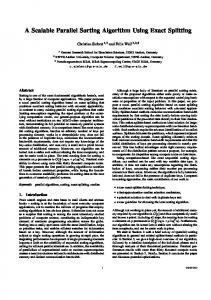
Figure 1: Recursive construction of multi-dimensional product networks: (a) the factor graph; (b) two-dimensional product; (c) three-dimensional product.
2 De nitions and Notation
2.1 De nitions and Notation Relating to Product Networks
Let G be an N -node connected graph, we de ne its r-dimensional homogeneous product as follows.
De nition 1 Given a graph G with vertex set VG = f0; 1; � � � ; N ? 1g and arbitrary edge set
EG , the r-dimensional homogeneous product of G, denoted PGr , is the graph whose vertex set is VPG = f0; 1; � � � ; N ? 1gr and whose edge set is EPG , de ned as follows: two vertices x = xr xr?1 � � � x1 and y = yr yr?1 � � � y1 are adjacent in PGr if and only if both of the following r
r
conditions are true: 1. x and y di�er in exactly one symbol position, 2. if i is the di�ering symbol index, then (xi ; yi ) 2 EG .
In this paper we assume that the r-tuple label for a node of PGr is indexed as 1 � � � r, with 1 referring to the rightmost position index and r referring to the leftmost position index. At a more intuitive level, the construction of PGr from PGr?1 , where PG1 = G, can be described by referring to Figure 1. Let x be a node of PGr?1, and let [u]PGr?1 be the graph obtained by pre xing every vertex x in PGr?1 by u, so that a vertex x becomes ux. First, place the vertices of PGr?1 along a straight line as shown in Figure 1. Then, draw N copies of PGr?1 such that the vertices with identical labels fall in the same column. Next extend the vertex labels to obtain [u]PGr?1, for u = 0; 1; � � � ; N ? 1. Finally, connect the columns in the interconnection pattern of the factor graph G, such that ux is connected to u0x if and only if (u; u0) 2 EG. In this construction, we use [u]PGr?1 to refer to the uth copy of PGr?1 . What is not explicitly stated here is the fact that [u]PGr?1 is the uth copy at dimension r. We can further extend this notation to allow us to add a new symbol at any position of the vertex labels. 4
For this purpose, we use [u]PGir?1 to mean that the vertex labels of PGr?1 are extended by inserting the value u at position i. As a result, the symbol at position j moves to position j + 1, where j = i; � � � ; r ? 1. De nition 1 allows us to observe that the construction of the preceding paragraph could be re-stated for [u]PGir?1 for any position i, not just the leftmost position. Conversely, we can obtain the [u]PGir?1 subgraphs, for u = 0; 1; � � � ; N ? 1, by erasing all the dimension-i edges in PGr . This process can be repeated recursively, and described by a simple extension of our notation: we use [u; v]PGi;j r?2 to refer to subgraphs isomorphic to PGr?2 obtained by erasing the connections at dimensions i and j from PGr . A particular subgraph so obtained can be distinguished by its unique combination of [u; v] values at index positions i and j , respectively. The notation is similarly extended for erasing arbitrary number of dimensions, and the order of the values in square brackets corresponds to the order of the superscripts.
2.2 De nition and Properties of the Sorted Order
For an arbitrary factor graph G, the vertex labels 0; � � � ; N ? 1 de ne the ascending order of data when sorted. However, we need to de ne an order for the nodes of PGr , which will determine the nal location of the sorted keys. The order de ned is known as snake order.
De nition 2 Snake order for the r-dimensional product graph PGr : 1. If r = 1, the snake order corresponds to the order used for labeling the nodes of G. 2. If r > 1, suppose that the snake order has been already de ned for PGr?1 . Then, (a) [u]PGrr?1 has the same order as PGr?1 if u is even, and reverse order if u is odd. (b) if u < v then any value in [u]PGrr?1 precedes any value in [v]PGrr?1 .
The snake order for product graphs is closely related to Gray-code sequences, which have the fundamental property that any two consecutive terms in the sequence di�er in exactly one bit. Here we are dealing with N -ary symbols instead of binary symbols. Therefore we need to use N -ary Gray-code sequences. First recall the de nition of Hamming distance and Hamming weight. Let s; z be r-tuples from f0; 1; � � � ; N ?1gr, then the Hamming distance between s and z is D(s; z) = Pri=1 jsi ?zij, where jsP i ? zij is the absolute value of si ? zi. The Hamming weight of an r-tuple s is W (s) = ri=1 si. Here we allow one or more of the elements of the r-tuples to be the special \all" symbol �, which will be de ned later. If any of the symbols in the r-tuple is the \all" symbol then its index position is omitted whenever the r-tuple is involved in the computation of Hamming distances and Hamming weights. We say that a sequence Qr is an N -ary Gray-code sequence of order r, if its elements are all the r-tuples in f0; 1; � � � ; N ? 1gr , and any two consecutive elements in it have unit Hamming distance. Consequently, the Hamming weights of two consecutive terms will have di�erent parity. We use R(Qr ) to denote the sequence obtained by listing the elements of Qr in reverse order. 5
The de nition below shows one way to construct N -ary Gray-code sequences of arbitrary order recursively. Let [u]Qk denote the sequence obtained by pre xing each element of Qk with the symbol u if u is even, or by pre xing each element of R(Qk ) with u, if u is odd.
De nition 3 An N -ary Gray-code sequence of order r, denoted Qr, can be obtained as 1. Q1 = f0; 1; � � � ; N ? 1g, 2. Qr = CON f[u]Qr?1 j u = 0; 1; � � � ; N ? 1g, where \CON fg" indicates concatenation of the sequences inside the curly brackets.
Note that Qr is in fact the snake order de ned on the vertices of the r-dimensional product network PGr .
Example: If N = 3, the 3-ary Gray-code sequences of order r, for r = 1, 2 and 3, are: � for r = 1, Q1 = f0; 1; 2g, � for r = 2, Q2 = f00; 01; 02; 12; 11; 10; 20; 21; 22g, � for r = 3, Q3 = f000, 001, 002, 012, 011, 010, 020, 021, 022, 122, 121, 120, 110, 111, 112, 102, 101, 100, 200, 201, 202, 212, 211, 210, 220, 221, 222g, Note that Qr could have been de ned for inserting the value u at any position in the above de nition, rather than the leftmost position. This observation allows us to use [u]Qir?1 to denote the subsequence of Qr that contains the value u in position i. We are especially interested in the subsequences [u]Q1r?1, for u = 0; � � � ; N ? 1. For given u, the elements of this subsequence are in positions u, 2N ? u ? 1, 2N + u, 4N ? u ? 1, 4N + u, and so on, in Qr . Given this observation, and the identity relationship between Qr and the snake order for the nodes of PGr , it follows that if PGr contains a sequence of keys sorted in snake order, the keys on the subgraph [u]PG1r?1 are also sorted in snake order, and are in the positions u, 2N ? u ? 1, 2N + u, 4N ? u ? 1, 4N + u, etc., of the whole sequence. Consider now dividing Qr into N r?1 subsequences of N consecutive elements each. We observe from De nition 3 that any two elements within the same subsequence would di�er in their rightmost symbols only. Thus, we can distinguish a particular subsequence of elements with the common symbols they have at positions 2; � � � ; r. We use [�]Q1r?1 to denote the group sequence obtained from Qr in this fashion, where � stands for all of 0; 1; � � � ; N ? 1. For example, given Q3 as above, its group sequence is [�]Q12 = f00�; 01�; 02�; 12�; 11�; 10�; 20�; 21�; 22�g where � stands for all of 0, 1, and 2. Thus, more explicitly, we can write [�]Q12 = f00[0; 1; 2]; 01[2; 1; 0]; 02[0; 1; 2]; 12[2; 1; 0]; 11[0; 1; 2]; 10[2; 1; 0]; 20[0; 1; 2]; 21[2; 1; 0]; 22[0; 1; 2]g: 6
Here, an element g of [�]Q1r?1 is of the form g = gr gr?1 � � � g2[Q1] if the Hamming weight of g is even, or of the form g = gr gr?1 � � � g2 [R(Q1)] if the Hamming weight of g is odd. Moreover, two successive elements of [�]Q1r?1 still have unit Hamming distance. Given the relation between Qr and PGr , an element g of [�]Q1r?1 identi es a dimension-1 G-subgraph of PGr . This is because in such a G-subgraph of PGr all node labels have the same values at symbol positions 2; � � � ; r. We say that a G-subgraph is even (resp. odd) if the Hamming weight for its corresponding element of [�]Q1r?1 is even (resp. odd). We ;1 to identify the set of PG -subgraphs at can extend the above notation and write [�; �]Q2r?2 2 ;1 will again have unit Hamming dimensions f1; 2g. Two consecutive elements of [�; �]Q2r?2 ;1 will be ordered in Gray-code sequence. Again, distance, and thus the elements of [�; �]Q2r?2 ;1 can have even or odd Hamming weight, and the corresponding an element g 2 [�; �]Qr2?2 PG2 subgraph can be said to be even or odd.
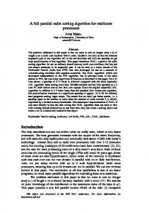
3 Multiway-Merge Sorting Algorithm This section develops the basic steps of the proposed sorting algorithm without regard to any speci c network. For this discussion, it does not even matter whether the algorithm is performed sequentially or in parallel. The subsequent sections will give the implementation details for product networks. A sorted sequence is de ned as a sequence of keys (a0; a1; � � � ; am?1) such that a0 � a1 � � � � � am?1. The multiway-merge algorithm combines N sorted sequences Ai = (ai;0; ai;1; � � � ; ai;m?1), for i = 0; � � � ; N ?1, into a single sorted sequence J = (j0; j1; � � � ; jmN ?1). Since this will be the case when we implement the algorithm on product networks, we will assume m to be some power of N , m = N k?1 , where k > 2, and hence the resulting sorted sequence, J , will contain N k keys. The heart of the proposed sorting algorithm is the multiway-merge operation. Thus, we will spend much of our time discussing this merging process. In order to build an intuitive understanding of the basic idea of the merge operation, we assume that the keys to be sorted are placed on a two-dimensional block, as shown in Figure 2. This is not to imply a two-dimensional organization of the data in product networks. When implementing the algorithm in product networks, each row of data (containing m = N k?1 keys) in Figure 2 will be stored on a (k ? 1)-dimensional subgraph of the product graph. The two-dimensional organization in Figure 2 is for the reader's convenience in visualizing what happens to the data at various steps of the algorithm, so that we can use the terms \row" and \column" in order to refer to groups of keys that are subjected to the same step of algorithm. Our use of the terms \row" and \column" should not be interpreted to imply the physical organization of data in a two dimensional array. Subject to this clari cation, we initially assume that each sorted sequence Ai, is in a di�erent row (see Figure 2). We also assume the existence of an algorithm which can sort N 2 keys. We make no assumption about the e�ciency of this algorithm as yet. In Section 5 we discuss several possible ways to obtain e�cient algorithms for this purpose. The purpose of this assumption is to maintain the generality of the discussions, independent of the factor network used to build the product network. To show the correctness of the algorithm we will use the zero-one principle due to Knuth 7
m=N
k-1
A0 A1 A2 . . . . . . .
N
A N-1
Figure 2: Initial situation before the merge process starts. Each sorted sequence is represented as a horizontal block (a row). [13]. The zero-one principle states that if an algorithm based on compare-exchange operations is able to sort any sequence of zeroes and ones, then it sorts any sequence of arbitrary keys.
3.1 Multiway-Merge Algorithm
Here we consider how to merge N sorted sequences, Ai = (ai;0; ai;1; � � � ; ai;m?1), for i = 0; � � � ; N ? 1, into a single large sorted sequence. The initial situation is pictured in Figure 2. The merge operation consists of the following steps:
Step 1: Distribute the keys of each sorted sequence Ai among N sorted subsequences Bi;j , for i = 0; � � � ; N ? 1 and j = 0; � � � ; N ? 1. The subsequence Bi;j will have the form (ai;j ; ai;2N ?j?1; ai;2N +j ; ai;4N ?j?1; ai;4N +j ; � � �), for i = 0; � � � ; N ? 1 and j = 0; � � � ; N ? 1. This is equivalent to writing the keys of each Ai on a Nm � N array in snake order (as shown in
Figure 3) and then reading the keys column-wise so that column j of the array becomes Bi;j , for j = 0; � � � ; N ? 1. Note that each subsequence Bi;j is sorted, since the keys in it are in the same relative order as they appeared in Ai. Figure 4 illustrates the situation after the completion of this process. Each of the N rows contains N sorted subsequences Bi;j , where each Bi;j box in Figure 4 corresponds to a column of keys in Figure 3 written horizontally.
Example: If for some i, Ai = f1; 2; 3; 4; 5; 6; 7; 8; 9g and N = 3, then Bi;0 = f1; 6; 7g; Bi;1 = f2; 5; 8g; Bi;2 = f3; 4; 9g; Step 2: Merge the N subsequences Bi;j found in column j of Figure 4 into a single sorted sequence Cj , for j = 0; � � � ; N ? 1. This is done in parallel for all columns by a recursive call to the multiway-merge process if the total number of keys in the column, m, is at least N 3. If the number of keys in a column of Figure 4 is N 2, a sorting algorithm for sequences of length N 2 is used (we already assumed the existence of such an algorithm above), because a recursive call to the merge process would not make much progress when m is N 2 (this point will be cleared at the end of this section). At the end of this step, we write the resulting subsequences vertically in N columns of length m each. The situation after this step is illustrated in Figure 5. 8
N
m/N
Bi,0
Bi,1
Bi,2
Bi,3
... B i,N-1
Figure 3: Distribution of the keys of Ai among the N subsequences Bi;j . The thick line represents the keys of Ai in snake order.
m/N
B 0,0
B 0,1
B 0,2
... ...
B 0,N-1 B 1,N-1
B 1,0
B 1,1
B 1,2
B 2,0
B 2,1
B 2,2
...
B 2,N-1
...
...
...
...
...
B N-1,0
B N-1,1
B N-1,2
...
B N-1,N-1
Figure 4: Situation after step 1: each sequence Ai, has been distributed into N subsequences Bi;j . Each of the subsequences contains m=N elements and is still sorted.
9
N
C0
C1
...
C2
C N-1
m
Figure 5: Situation after merging the subsequences in each column. The keys are sorted from top to bottom.
Step 3: Interleave the sequences Cj into a single sequence D = (d0; d1; � � � ; dmN ?1). The sequence D is formed simply by reading the m � N array of Figure 5 in row-major order
starting from the top row. The sequence D is re-drawn in Figure 6 from the Cj sequences of Figure 5 with no change in the organization of data. Figure 6 is identical to Figure 5, except that we regard it as one big sequence to be read in row-major order. We prove below that D is now \almost" sorted. This situation is shown in Figure 6. If the keys being sorted can only take values of zero or one, the shaded area represents the position of zeroes and the white area represents the position of ones. As D is obtained by reading the values in row-major order, the potential dirty area (window of keys not sorted) has length no larger than N 2. This fact will be shown in Lemma 1.
Step 4: Clean the dirty area. To do so we start by dividing the sequence D into m=N subsequences of N 2 consecutive keys each. We denote these subsequences as Ei, for i = 0; � � � ; Nm ? 1. The ith subsequence has the form Ei = (diN ; diN +1; � � � ; diN +N ?1). That is, 2
2
2
2
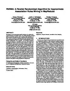
the rst N rows of keys in Figure 6 (or equivalently in Figure 5) are concatenated to obtain E1, the next N rows are concatenated to obtain E2, and so on (see Figure 7.(a)). We then independently sort the subsequences (rows in Figure 7.(a)) in alternate orders by using the algorithm which we assumed available for sorting N 2 keys. Ei is transformed into a sequence Fi (see Figure 7.(b)), where Fi contains the keys of Ei sorted in non-decreasing order if i is even or in non-increasing order if i is odd, for i = 0; � � � ; Nm ? 1. Now, we apply two steps of odd-even transposition between the sequences Fi, for i = 0; � � � ; Nm ? 1 (i.e. in the vertical direction of Figure 7.(b)). In the rst step of odd-even transposition, each pair of sequences Fi and Fi+1, for i even, are compared element by element. Two sequences Gi and Gi+1 are formed (not shown in the gure) where gi;k = minffi;k ; fi+1;k g and gi+1;k = maxffi;k; fi+1;k g. In the second step of the odd-even transposition, Gi and Gi+1 10
m N rows (dirty)
N
Figure 6: Sequence D obtained after interleaving. The order goes from top to bottom by reading successive rows from left to right. The shaded area is lled with zeroes and the white area is lled with ones. The boundary area has at most N rows, as shown in Lemma 1. for i odd are compared in a similar manner to form the sequences Hi and Hi+1. Figure 7.(c) shows the situation after the two steps of odd-even transposition. Finally, we sort each sequence Hi in non-decreasing order, generating sequences Ii, for i = 0; � � � ; Nm ? 1 (see Figure 7.(d)). The nal sorted sequence J is the concatenation of the sequences Ii. We need to show that the process described actually merges the sequences. To do so we use the zero-one principle mentioned earlier.
Lemma 1 When sorting an input sequence of zeroes and ones, the sequence D obtained
after the completion of step 3 is sorted except for a dirty area which is never larger than N 2 .
Proof: Assume that we are merging sequences of zeroes and ones. Let zi be the number of zeroes in sequence Ai, for i = 0; � � � ; N ? 1. The rest of keys in Ai are ones. Step 1 breaks each sequence Ai into N subsequences Bi;j , j = 0; � � � ; N ? 1. It is easy to observe, from the way step 1 is implemented, that the number of zeroes in a subsequence Bi;j is bzi=N c + qij , where qij is either 0 or 1. Therefore, for a given i, the sequences Bi;j can di�er from each other in their number of zeroes by at most one. At the start of step 2, each column j is composed of the subsequences Bi;j for i = 0; � � � ; N ? 1. At the end of step 2, all the zeroes are at the beginning of each sequence Cj . The number of zeroes in each sequence Cj is the sum of the number of zeroes in Bi;j for xed j and i = 0; � � � ; N ? 1. Thus, two sequences Cj can di�er from each other by at most N zeroes. In step 3 we interleave the N sorted sequences into the sequence D by taking one key at a time from each sequence Cj . Since any two sequences Cj can di�er in their number of zeroes by at most N , and since there are N sequences being interleaved, 11
(a)
E0 E1
(b)
(c)
(d)
F0 F1
H0 H1
I0 I1
N k-2
N
2
Figure 7: Cleaning of the dirty area. the length of the window of keys where there is a mixture of ones and zeroes is at most N 2. Now we can show how the last step actually cleans the dirty area in the sequence. Lemma 2 The sequence J obtained (by concatenation of sequences Ii in snake order) after the completion of step 4 is sorted. Proof: We know that the dirty area of the sequence D, obtained in step 3, has at most length N 2. If we divide the sequence D into consecutive subsequences, Ei, of N 2 keys each, the dirty area can either t in exactly one of these subsequences or be distributed between two adjacent subsequences. If the dirty area ts in one subsequence Ek , then after the initial sorting and the oddeven transpositions, the sequences Hi contain exactly the same keys as the sequences Ei, for i = 0; � � � ; Nm ? 1. Then, the last sorting in each sequence Hi and the nal concatenation of the Ii sequences yield a sorted sequence J . However, if the dirty area is distributed between two adjacent subsequences, Ek and Ek+1 , we have two subsequences containing both zeroes and ones. Figure 7.(a) presents an example of this initial situation. After the rst sorting, the zeroes are located at one side of Fk and at the other side of Fk+1 (see Figure 7.(b)). One of the two odd-even transpositions will not a�ect this distribution, while the other is going to move zeroes from the second sequence to the rst and ones from the rst to the second. After these two steps, Hk is lled with zeroes or Hk+1 is lled with ones (see Figure 7.(c)). Therefore, only one sequence contains zeroes and ones combined. The last step of sorting will sort this sequence. Then the entire sequence J will be sorted (see Figure 7.(d)).
3.2 The Need for a Special Algorithm for N 2 Keys
The reader can observe that, at the end of step 3, the dirty area will still have length N 2 even when we are merging N sequences of length N each. Thus, we do not make much progress 12
when we apply the multiway-merge process to this case. This is a fundamental property of the merge process, and not a weakness of our algorithm. This di�culty can be overcome in a number of ways to keep the running time low, depending on the application area of the basic idea of the merge algorithm. For example, if we are interested in building a sorting network, we can implement subnetworks based on recursively updating N to a smaller value M and then merge M sequences of length M k?1 = N for some k > 2, and repeat this recursion until a single sequence is obtained. In this paper our focus is developing sorting algorithms for product networks. Here we assume the availability of a special sorting algorithm designed for the two-dimensional version of the product network under consideration. In subsequent sections we discuss several methods to obtain such algorithms as we consider more speci c product networks. The e�ciency of that special algorithm has an important e�ect on the overall complexity of the nal sorting algorithm by the proposed approach. For all the cases considered here, it will turn out that the resulting running time is either asymptotically optimal or close to optimal when the number of dimensions is bounded.
3.3 Sorting Algorithm
Using the above algorithm, and an algorithm to sort sequences of length N 2, it is easy to obtain a sorting algorithm to sort a sequence of length N r , for r � 2. First divide the sequence into subsequences of length N 2 and sort each subsequence independently. Then, apply the following process until only one sequence remains: 1. Group all the sorted sequences obtained into sets of N sequences each as in Figure 1. (If we are sorting N r keys, then initially there will be N r?3 groups, each containing N sorted sequences of length N 2.) 2. Merge the sequences in each group into a single sorted sequence using the algorithm shown in the previous section. If now there is only one sorted sequence then terminate. Otherwise go to step 1.
4 Implementation on Homogeneous Product Networks Here we mainly focus on the implementation of the multiway-merge algorithm on a kdimensional product network PGk in detail. The sorting algorithm trivially follows from the merge operation as described above. The initial scenario is N sorted sequences, of N k?1 keys each, stored on the N subgraphs [u]PGkk?1 of PGk in snake order. Before the sorting algorithm starts each processor holds one of the keys to be sorted. During the sorting algorithm, each processor needs enough memory to hold at most two values being compared. Throughout the discussions, the steps of implementation are illustrated by a three-dimensional product of some graph G of N = 3 nodes. The interconnection pattern of G is irrelevant for this discussion.
Step 1: This step does not need any computation or routing. Recall from Section 2 that k;1
each of the subgraphs [u; v]PGk?2 of [u]PGkk?1 contains a subsequence of keys sorted in snake 13
dimension 3 dimension 1
dimension 2
0
4
4
1
4
5
0
0
1
7
5
5
6
5
5
2
1
1
8
8
9
7
7
8
3
4
9
Figure 8: Initial situation on the example 3-dimensional product graph. dimension 1 dimension 3
(a)
dimension 2
0
1
0
4
4
0
4
5
1
7
6
2
5
5
1
5
5
1
8
7
3
8
7
4
9
8
9
dimension 1 dimension 3
(b)
dimension 2
0
6
7
0
5
5
1
5
8
0
3
7
1
4
7
1
5
9
1
2
8
4
4
8
4
5
9
Figure 9: Step 2 of the multiway-merge algorithm. order, and that the positions of the keys in that subsequence with respect to the total sorted sequence are v, 2N ? v ? 1, 2N + v, 4N ? v ? 1, 4N + v, etc. Therefore, the sequence Bu;v 1 , sorted in snake order. is already stored on the subgraph [u; v]PGk;k?2 This is illustrated in Figure 8, where the three sequences to be merged are available in snake order on the three subgraphs formed by removing the edges of dimension-3. The subgraph [0]PG32 (leftmost subgraph in Figure 8) contains A0, the subgraph [1]PG32 (center subgraph) contains A1, and the subgraph [2]PG32 (rightmost subgraph) contains A2. In this example, each Bu;v contains only N keys, which t in just one G subgraph. In general, Bu;v 1 . In this example, they are at [u; v ]PG3;1, will be available in snake order on [u; v]PGk;k?2 1 which really correspond to G-subgraphs at dimension 2 (i.e. columns of Figure 8).
Step 2: This step is implemented by merging together the sequences on subgraphs [u; v]PGk;k?21 with the same u value into one sequence on [v]PG1k?1. If k ? 1 = 2, the merging is done by directly sorting with an algorithm for PG2. If k ? 1 > 2, this step is done by a recursive call to the multiway-merge algorithm, where each subgraph [v]PG1k?1 merges the sorted 14
dimension 3 dimension 1
dimension 2
0
0
1
6
5
5
7
5
8
0
1
1
3
4
5
7
7
9
1
4
4
2
4
5
8
8
9
Figure 10: Step 3 of the multiway-merge algorithm. 1 subgraphs. sequences stored on their [u; v]PGk;k?2 We illustrate this step in Figure 9. For clarity, we rst show the initial situation in Figure 9.(a). This is same as the situation in Figure 8, but dimensions 1 and 3 are exchanged to show the subsequences that will be merged together more explicitly. The Bu;v sequences to be merged together are the columns of Figure 9.(a). The result of merging is shown in Figure 9.(b). Each Cv is sorted in snake order and is found in the subgraph [v]PG12.
Step 3: This step is directly done by reintroducing the dimension-1 connections of PGk
and reading the keys in snake order for the PGk graph. No movement of data is involved in this step. We explicitly show the resulting sequence for our example in Figure 10 by switching dimensions 1 and 3 in Figure 9.(b). The reader can observe from Figure 10 that the keys now appear to be close to a fully sorted order (compare Figure 10 with Figure 11.d which shows the nal sorted order). In fact, we know from Lemma 1 that in the case of sorting zeroes and ones, we are left with a small dirty area. This implies that every key is within a distance of N 2 from its nal position.
Step 4: This last stepk;cleans the potential dirty area. Recall that the 2-dimensional ��� ; 3 1, subgraphs [uk � � � ; u3]PG2 of PGk can be identi ed by the group sequences [�; �]Q2k;?2 1 identi es a unique PG subgraph at dimensions f1; 2g, and that an element g of [�; �]Q2k;?2 2
that these PG2 subgraphs are ordered by the corresponding group sequence which de nes the snake order between subgraphs. In this step we independently sort the keys in each PG2 subgraphs at dimensions f1; 2g, where the sorted order alternates for \consecutive" subgraphs. Each subgraph is sorted in snake order by using an algorithm which we assumed available for two dimensions. The result of this step is illustrated in Figure 11.(a). We now perform two steps of odd-even transposition between the subgraphs. In the rst step, the keys on the nodes of the \odd" PG2 subgraphs are compared with the keys on the corresponding nodes of their \predecessor" subgraphs. The keys are exchanged if the key in the predecessor subgraph is larger. Figure 11.(b) shows the result of this rst step in our example. The keys 3 and 2 in nodes (1; 2; 1) and (1; 2; 2) have been exchanged with two keys both with value 4 in nodes (0; 2; 1) and (0; 2; 2). In the second step of odd-even transposition, the keys on the nodes of the \even" PG2 subgraphs are compared (and possibly exchanged ) with those of their predecessor subgraphs. Figure 11.(c) shows the result of this second step. In this gure, the key 5 in node (2,0,0) has been exchanged with the key 6 in node (1,0,0). 15
dimension 3 dimension 1
(a)
dimension 2
0
0
0
6
5
5
5
7
7
1
1
1
4
5
5
8
8
7
1
4
4
4
3
2
8
9
9
dimension 3 dimension 1
(b)
dimension 2
0
0
0
6
5
5
5
7
7
1
1
1
4
5
5
8
8
7
1
3
2
4
4
4
8
9
9
dimension 3 dimension 1
(c)
dimension 2
0
0
0
5
5
5
6
7
7
1
1
1
4
5
5
8
8
7
1
3
2
4
4
4
8
9
9
dimension 3 dimension 1
(d)
dimension 2
0
0
0
5
5
5
6
7
7
1
1
1
4
5
5
8
8
7
1
2
3
4
4
4
8
9
9
Figure 11: Step 4 of the multiway-merge algorithm.
16
Finally, a sorting within each of the 2-dimensional subgraphs ends the merge process (Figure 11.(d)). One point which needs to be examined in more detail here is that, depending on the factor graph G, the nodes holding the two keys that need to be compared and possibly exchanged with each other may or may not be adjacent in PGk . If G has a Hamiltonian path, then the nodes of G can be labeled in the order they appear on the Hamiltonian path to de ne the sorted order for G. Then, the two steps of odd-even transposition are easy to implement since they involve communication between adjacent nodes in PGk . If, however, G is not Hamiltonian (e.g. a complete binary tree), the two nodes whose keys need to be compared may not be adjacent, but they will always be in a common G subgraph. In this case permutation routing within G may be used to perform the compare-exchange step as follows: First, two nodes that need to compare their keys send their keys to each other. Then, depending on the result of comparison, each node can either keep its original key if the keys were already in correct order, or they drop the original key and keep the new key if they were out of order. To cover the most general case in the computation of running time below, we will assume that G is not Hamiltonian, and thus we will implement these compare-exchange steps by using permutation routing algorithms. We will see that whether or not G is Hamiltonian only e�ects the constant terms in the running time complexity function.
4.1 Analysis of Time Complexity
To analyze the time taken by the sorting algorithm we will initially study the time taken by the merge process on a k-dimensional network. This time will be denoted as Mk (N ). Also let S2(N ) denote the time required for sorting on PG2 and R(N ) denote the time required for a permutation routing on G.
Lemma 3 Merging N sorted sequences of N k?1 keys on PGk takes Mk (N ) = 2(k?2)(S2 (N )+ R(N )) + S2(N ) time steps.
Proof: Step 1 does not take any computation time. Step 2 is a recursive call to the merge procedure for k ? 1 dimensions, and hence will take Mk?1(N ) time. Step 3 does not take any computation time. Finally, step 4 takes the time of one sorting on PG2 , two permutation routings on G (for the steps of odd-even transposition), and one more sorting on PG2. Therefore, the value of Mk (N ) can be recursively expressed as: Mk (N ) = Mk?1 (N ) + 2(S2(N ) + R(N )) with initial condition that yields
M2(N ) = S2(N ) Mk (N ) = 2(k ? 2)(S2(N ) + R(N )) + S2(N )
We can now derive the value of Sr (N ). 17
Theorem 1 For any factor graph G, the time complexity of sorting N r keys on PGr is Sr (N ) = (r ? 1)2S2(N ) + (r ? 1)(r ? 2)R(N ) = O(r2 S2(N )). Proof: By the algorithm of Section 3.2 the time taken to sort N r keys on PGr is the time taken to sort in a 2-dimensional subgraph and then merge blocks of N sorted sequences into increasing number of dimensions. The expression of this time is as follows: Sr (N ) = S2(N ) + M3(N ) + M4(N ) + � � � + Mr?1(N ) + Mr (N )
Xr
= (r ? 1)S2(N ) + 2(S2(N ) + R(N )) (i ? 2) i=3
= (r ? 1)2S
2 (N ) + (r ? 1)(r ? 2)R(N ):
Since S2(N ) is never smaller than R(N ), the time obtained is Sr (N ) < 2(r ? 1)2S2(N ) = O(r2 S2(N )). The following corollary presents the asymptotic complexity of the algorithm and one of the main results of this paper. Corollary 1 If G is a connected graph, the time complexity of sorting N r keys on PGr is at most 18(r ? 1)2N + o(r2 N ) = O(r2 N ). Proof: To prove the claim, we rst compute the complexity of sorting by our algorithm on the r-dimensional torus. Then we refer to a result in [8] that showed that if G is a connected graph, PGr can emulate any computation on the N r -node r-dimensional torus by embedding the torus into PGr with dilation 3 and congestion 2. Since this embedding has constant dilation and congestion, the emulation has constant slowdown [14]. (In fact, the slowdown is no more than 6, and needed only when G does not have a Hamiltonian cycle). Finally, we use these slowdown values to compute the exact running time for PGr Now we compute the complexity of sorting on the r-dimensional torus. We basically need a sorting algorithm from the literature that sorts N 2 keys in two-dimensional torus in snake order. We also need an algorithm for permutation routing on the N -node cycle. For example, we can use the sorting algorithm proposed by Kunde [15], which has complexity 2:5N + o(N ). It is also known that any permutation routing can be done on the N -node cycle in no more than N=2 steps. Hence, we can sort on the N r -node r-dimensional torus in at most 3(r ? 1)2N + o(r2 N ) steps. Since the emulation of this algorithm by PGr requires a slowdown factor of at most 6, any arbitrary N r -node r-dimensional product network can sort with complexity 18(r ? 1)2N + o(r2N ) = O(r2 N ).
5 Application to Speci c Networks In this section we obtain the time complexity of sorting using the multiway-merge sorting algorithm presented for several product networks in the literature. To do so, we obtain upper bounds for the values of S2(N ) and R(N ) for each network. Using these values in Theorem 1 will yield the desired running time. 18
Grid: Schnorr and Shamir [29] have shown that it is possible to sort N 2 keys on a N 2-node 2-dimensional grid in 3N + o(N ) time steps. It is also trivial to show that the time to perform a permutation on the N -node linear array is at most R(N ) = N ? 1. These values of S2(N ) and R(N ) imply that our algorithm will take at most 4(r ? 1)2N + o(r2N ) = O(r2N ) time steps to sort N r keys on an N r -node r-dimensional grid. If the number of dimensions, r, is bounded, this expression simpli es to O(N ). This algorithm is asymptotically optimal when r is xed since the diameter of the grid with bounded number of dimensions is O(N ), and a value may need to travel as far as the diameter of the network. If r is not bounded, then the diameter of the N r -node grid is r(N ? 1), which means that the running time of our algorithm is o� the optimal value by at most a factor of r.
Mesh-connected trees (MCT): This network was introduced in [9] and extensively studied in [8]. It is obtained as the product of complete binary trees. Due to Corollary 1 we can sort on the N r -node r-dimensional mesh-connected trees in O(r2 N ) time steps. If r is bounded, we again have O(N ) as the running time. This running time is asymptotically optimal when r is xed, because the bisection width of the N r -node r-dimensional MCT is O(N r?1 ), as shown in [8], and in the worst case we may need to move (N r ) values across the bisection of the network. When r is not xed, the algorithm is o� the bisection-based lower bound by a factor of r2. The diameter-based lower bound used above for grids does not help to tighten this lower bound any further, because the diameter of the MCT is logarithmic in the number of nodes [8]. It appears interesting to investigate if it is possible to sort with lower running time than O(r2N ) when r is not bounded. If such an algorithm exists, it must use a completely di�erent approach than ours, because the value of S2(N ) in Theorem 1 cannot be less than O(N ) due to the O(N ) bisection width of the two-dimensional MCT network.
Hypercube: The hypercube has xed N = 2. It is not hard to sort in snake order on
the two-dimensional hypercube in 3 steps. A permutation routing on the one-dimensional hypercube takes only one step. Therefore, the time to sort on the hypercube with our algorithm is 3(r ? 1)2 + (r ? 1)(r ? 2) = O(r2 ). This running time is same as the running time of the well-known Batcher odd-even merge algorithm for hypercubes. In fact, Batcher algorithm is a special case of our algorithm.
Petersen Cube: The Petersen cube is the r-dimensional product of the Petersen graph,
shown in Figure 12. The Petersen graph contains 10 nodes and consists of an outer 5-cycle and an inner 5-cycle connected by ve spokes. Product graphs obtained from the Petersen graph are studied in [25]. Like the hypercube, the product of Petersen graphs has xed N , and therefore the only way the graph grows is by increasing the number of dimensions. Since the Petersen graph is Hamiltonian, its two-dimensional product contains the 10 � 10 two-dimensional grid as a subgraph. Thus, we can use any grid algorithm for sorting 100 keys on the two-dimensional product of Petersen graphs in constant time. Consequently, the r-dimensional product of Petersen graphs can sort 10r keys in O(r2 ) time. The constant involved is not small, but it is not going to be unreasonably large either. It may very well 19
Figure 12: Petersen graph. be possible to improve this constant by developing a special sorting algorithm for the twodimensional product of Petersen graphs. This is, however, outside the scope of this paper.
Product of de Bruijn and shu�e-exchange networks: To sort on their two-dimensional instances we can use the embeddings of their factor networks presented in [9] which have small constant dilation and congestion. In particular, a N 2-node shu�e-exchange network can be embedded into the N 2-node 2-dimensional product of shu�e-exchange networks with dilation 4 and congestion 2. Also a N 2-node de Bruijn network can be embedded into the N r -node 2-dimensional product of de Bruijn networks with dilation 2 and congestion 2. Sorting N 2 keys on the N 2-node shu�e-exchange or de Bruijn networks can be done in O(log2 n) time by using Batcher algorithm [30]. Thus, we can sort on the N 2-node 2-dimensional product of shu�e-exchange or de Bruijn network by emulation of the N 2-node shu�e-exchange or de Bruijn network in S2(N ) = O(log2 N 2) = O(log2 N ) time steps. Using this in Theorem 1, our algorithm will take O(r2 log2 N ) time steps to sort N r keys. Again, if r is bounded the expression simpli es to O(log2 N ). If r is not bounded, the running time of our algorithm is asymptotically the same as the running time of sorting N r keys on the N r -node de Bruijn or shu�e-exchange graphs by Batcher algorithm. Here again, we come across an interesting open problem, to see if it is possible to sort on products of these networks in asymptotically less time for unbounded number of dimensions.
6 Conclusions In this paper we have presented a uni ed approach to sorting on homogeneous product networks. To do so, we present an algorithm based on a generalization of the odd-even merge sorting algorithm [2]. We obtain O(r2 N ) as an upper bound on the complexity of sorting on any product network of r dimensions and N r nodes. The time taken by the sorting algorithm on the grid and the mesh-connected trees with bounded number of dimensions is O(N ), which is optimal. On the hypercube the algorithm takes O(r2 ) time steps, reaching the asymptotic complexity of the odd-even merge sorting algorithm on the hypercube. On other product networks our algorithm has the same running time as those of other comparable networks. For instance, on the product of de Bruijn or shu�e-exchange graphs the running time is O(r2 log2 N ). This is asymptotically the same as the running time of Batcher algorithm on the N r -node shu�e-exchange or de Bruijn graphs. From a theoretical point of view, it will be interesting to investigate if there are better algorithms for product networks when r is not bounded. Several interesting alternatives 20
appear to be feasible, although we have not had the time to investigate them. For instance, we could try to generalize the hypercube randomized algorithms for product networks.
References [1] A. Aggarwal and M.-D. A. Huang, \Network Complexity of Sorting and Graph Problems and Simulating CRCW PRAMS by Interconnection Networks," in Proceedings of the 3rd Aegean Workshop on Computing, AWOC 88: VLSI Algorithms and Architectures (J. H. Reif, ed.), vol. 319 of Lecture Notes in Computer Science, pp. 339{350, Corfu, Greece: Springer Verlag, July 1988. [2] K. Batcher, \Sorting Networks and their Applications," in Proceedings of the AFIPS Spring Joint Computing Conference, vol. 32, pp. 307{314, 1968. [3] K. E. Batcher, \On Bitonic Sorting Networks," in Proceedings of the 1990 International Conference on Parallel Processing, vol. I, 1990, pp. 376-379. [4] M. Baumslag and F. Annexstein, \A Uni ed Framework for O�-Line Permutation Routing in Parallel Networks," Math. Systems Theory, vol. 24, no. 4, pp. 233{251, 1991. [5] G. E. Blelloch, C. E. Leiserson, B. M. Maggs, C. G. Plaxton, S. Smith, and M. Zagha, \A Comparison of Sorting Algorithms for the Connection Machine CM-2," in Proceedings of the 3rd Annual ACM Symposium on Parallel Algorithms and Architectures, pp. 3{16, July 1991. [6] R. Cypher and C. G. Plaxton, \Deterministic Sorting in Nearly Logarithmic Time on the Hypercube and Related Computers," Journal of Computer and System Sciences, vol. 47, pp. 501{548, Dec. 1993. [7] R. L. S. Drysdale III and F. H. Young, \Improved Divide/Sort/Merge Sorting Network," SIAM Journal on Computing, vol. 4, pp. 264{270, Sept. 1975. [8] K. Efe and A. Fern�andez, \Computational Properties of Mesh Connected Trees: Versatile Architecture for Parallel Computation," in Proceedings of the 1994 International Conference on Parallel Processing, vol. I, (St. Charles, IL), pp. 72{76, CRC Press Inc., Aug. 1994. [9] K. Efe and A. Fern�andez, \Products of Networks with Logarithmic Diameter and Fixed Degree," IEEE Transactions on Parallel and Distributed Systems, vol. 6, pp. 963{975, Sept. 1995. [10] T. El-Ghazawi and A. Youssef, \A General Framework for Developing Adaptive FaultTolerant Routing Algorithms," IEEE Transactions on Reliability, vol. 42, pp. 250{258, June 1993. [11] A. Fern�andez, Homogeneous Product Networks for Processor Interconnection. PhD thesis, U. of Southwestern Louisiana, Lafayette, LA, Oct. 1994. 21
[12] M. W. Green, \Some Improvements in Non-Adaptative Sorting Algorithms," in Proceedings of the 6th Princeton Conference on Information Sciences and Systems, pp. 387{391, 1972. [13] D. Knuth, Searching and Sorting, vol. 3 of The Art of Computer Programming. Reading, MA: Addison-Wesley, 1973. [14] R. Koch, T. Leighton, B. Maggs, S. Rao, and A. L. Rosenberg, \Work-Preserving Emulations of Fixed-Connection Networks," in Proceedings of the 21st Annual ACM Symposium on Theory of Computing, (Seattle), pp. 227{240, May 1989. [15] M. Kunde, \Optimal Sorting on Multi-Dimensionally Mesh-Connected Computers," in Proceedings of the 4th Annual Symposium on Theoretical Aspects of Computer Science (F. J. Brandenburg, G. Vidal-Naquet, and M. Wirsing, eds.), vol. 247 of Lecture Notes in Computer Science, pp. 408{419, Springer Verlag, 1987. [16] D.-L. Lee and K. E. Batcher, \A Multiway Merge Sorting Network," IEEE Transactions on Parallel and Distributed Systems, vol. 6, pp. 211{215, Feb. 1995. [17] D.-L. Lee and K. E. Batcher, \On Sorting Multiple Bitonic Sequences," in Proceedings of the 1994 International Conference on Parallel Processing, vol. I, August 1994, pp. 121-125. [18] F. T. Leighton, Introduction to Parallel Algorithms and Architectures: Arrays, Trees, and Hypercubes. San Mateo: Morgan Kaufmann, 1992. [19] T. Leighton, \Tight Bounds on the Complexity of Parallel Sorting," IEEE Transactions on Computers, vol. C-34, pp. 344{354, Apr. 1985. [20] K. J. Liszka and K. E. Batcher, \A Modulo Merge Sorting Network," in Proceedings of the Fourth Symposium on the Frontiers of Massively Parallel Computation, (McLean, VA), pp. 164{169, IEEE Computer Society Press, Oct. 1992. [21] K. J. Liszka and K. E. Batcher, \A Generalized Bitonic Sorting Network," in Proceedings of the 1993 International Conference on Parallel Processing, vol. I, pp. 105{108, Aug. 1993. [22] D. Nassimi and S. Sahni, \Bitonic Sort on a Mesh-Connected Parallel Computer," IEEE Transactions on Computers, vol. C-27, pp. 2{7, Jan. 1979. [23] T. Nakatani, S.-T. Huang, B. W. Arden, and S. K. Tripathi, \K-Way Bitonic Sort," IEEE Transactions on Computers, vol. 38, no. 2, February 1989, pp. 283{288. [24] D. Nath, S. N. Maheshwari, and P. C. P. Bhatt, \E�cient VLSI Networks for Parallel Processing Based on Orthogonal Trees," IEEE Transactions on Computers, vol. C-32, pp. 569{581, June 1983. [25] S. R. Ohring and S. K. Das, \The Folded Petersen Network: A New CommunicationE�cient Multiprocessor Topology," in Proceedings of the 1993 International Conference on Parallel Processing, vol. I, pp. 311{314, Aug. 1993. 22
[26] B. Parker and I. Parberry, \Constructing Sorting Networks from k-Sorters," Information Processing Letters, vol. 33, pp. 157{162, Nov. 1989. [27] F. Preparata and J. Vuillemin, \The Cube-Connected Cycles: A Versatile Network for Parallel Computation," Communications ACM, vol. 24, pp. 300{309, May 1981. [28] A. L. Rosenberg, \Product-Shu�e Networks: Toward Reconciling Shu�es and Butter ies," Discrete Applied Mathematics, vol. 37/38, pp. 465{488, July 1992. [29] C. P. Schnorr and A. Shamir, \An Optimal Sorting Algorithm for Mesh Connected Computers," in Proceedings of the 18th Annual ACM Symposium on Theory of Computing, (Berkeley, CA), pp. 255{263, May 1986. [30] H. Stone, \Parallel Processing with the Perfect Shu�e," IEEE Transactions on Computers, vol. C-20, pp. 153{161, Feb. 1971. [31] C. D. Thompson and H. T. Kung, \Sorting on a Mesh-Connected Parallel Computer," Communications ACM, vol. 20, pp. 263{271, Apr. 1977. [32] S. S. Tseng and R. C. T. Lee, \A Parallel Sorting Scheme whose Basic Operation Sorts n Elements," International Journal Computer and Information Sciences, vol. 14, no. 6, pp. 455{467, 1985. [33] D. C. V. Voorhis, \An Economical Construction for Sorting Networks," in Proceedings of the AFIPS National Computer Conference, vol. 43, pp. 921{927, 1974.
23