Basic Theory. Traditional cross- ...... 1 Introduction. Part I (Belmont and Hotchkiss, 1997), develops the basic ..... traditional linear programming methods or the ...
Generalized
M. R. Belmont School of Engineering, University of Exeter, Harrison Engineering Building, North Park Road, Exeter EX4 4QF, UK
A. J. Hotchkiss Sun Electric Europe Research
Functions for Engineering Applications, Part I: Basic Theory Traditional cross-correlation considers situations where two functions or data sets are linked by a constant shift either in time or space. Correlation provides estimates of such shifts even in the presence of considerable noise corruption. This makes the technique valuable in applications like sonar, displacement or velocity determination and pattern recognition. When regions are decomposed into patches in applications such as Particle Image Velocimerty it also allows estimates to be made of whole displacement/flow fields. The fundamental problem with traditional correlation is that patch size and hence statistical reliability must be compromised with resolution. This article develops a natural generalization of cross-correlation which removes the need for such compromises by replacing the constant shift with a function of time or space. This permits correlation to be applied globally to a whole domain retaining any long-range coherences present and dramatically improves statistical reliability by using all the data present in the domain for each estimate.
1 Introduction The cross-correlation of two function or data sets fl and f2 (Weiner, 1949, 1964) is a very common tool in applications as diverse as sonar, flow determination, and pattern recognition in badly corrupted data (Trahey et a!., 1969; Coupland and Halliwell, 1992; Richards and Roberts, 1971; Lee, 1960; Matic et a!., 1991; Berryman and Blair, 1986; Dejong et a!., 1991; Gonzalez and Woods, 1992). Conventional cross-correlation typically applies to situations where the quantities of interestfl and f2 are related by a simple constant shift T: f2m=fl(~+T)
(1)
and the aim is to obtain a statistically reliable estimate of what will be termed here the transformation parameter T. In time series work ~ is the time t and T a time delay while in spatial applications ~ and T define N dimensional displacement vectors, rotations, or some combination of these (Gonzalez and Woods, 1992; Kamachi, 1989). For applications like particle image velocimetry (Willert and Gharib, 1991; Utami et aI., 1991; Adrian, 1986), where a whole flow field is characterized, cellular correlation has been developed (Kamachi, 1989; Leese et a!., 1971; Ninnis et a!., 1986). The displacement/flow field is made visible in some way with fl and f2 being consecutive images of the displacement/flow. The images are segmented into patches and cross-correlation is then' applied essentially to each patch in turn to determine an average displacement/flow velocity for each such cell. The main problem with this approach is that increasing spatial resolution means reducing the patch size. As typical applications involve digitized noise corrupted data this reduces the information available in each patch for correlation and thus degrades
Contributed by the Applied Mechanics Division of THE AMERICAN SOCIETY OF MECHANICAL ENGINEERS for publication in the AS ME JOURNAL OF ApPLIED MECHANICS. Discussion on Ihe paper should be addressed to the Technical Editor, Professor Lewis T. Wheeler, Department of Mechanical Engineering, University of Houston, Houston, TX 77204-4792, and will be accepted until four months after final publication of the paper itself in the ASME JOURNAL OF ApPLIED MECHANICS. Manuscript received by the AS ME Applied Mechanics Division, Sept. 27. \995: final revision, Oct. 28, 1996. Associate Technical Editor: S. Lichter.
Journal of Applied Mechanics
Cross-Correlation
the reliability of the estimates. If the noise is Gaussian variance of the sample estimate is inversely proportional to patch size. Furthermore, treating each cell independently loses the information theoretic advantages stemming from intercellular coherence in the displacement/flow field. These problems could be avoided if cross-correlation could be generalized to allow spatial or temporal variation of the shift T and the present article is concerned with developing such a Generalized Cross-Correlation (denoted as GC-C). The range of uses of conventional cross-correlation extends far beyond the description of displacement/flow problems cited here in both practical and analytical areas, and consequently the scope of GC-C is expected to be even wider. The treatment here in Part I is in terms of continuous variables while issues associated with discretisation are addressed in the companion work Part II, Belmont et al. (1997).
2 The Properties Required of a Cross-Correlation Function The first step in developing the GC-C is to specify those features which a cross-correlation function of any kind should exhibit. These are natural extensions of the characteristics exhibited by conventional cross-correlation (Weiner, 1949, 1964): . 1 Cross-correlation should operate upon a pair of functions, or data sets, (in its discrete form), denoted as fl and f2. 2 If fI and f2 are connected by some transformation of their independent variables, then the cross-correlation function should exhibit an absolute maximum when a matching transformation is induced by cross-correlation processes. A corollary of this is that the location of the maximum should allow the computation of any parameters associated with the transformation, e.g., T in Eq. (1). 3 The cross-correlation function should approach the absolute maximum smoothly. 4 Points 2 and 3 should hold even iffl and f2 are contaminated by extraneous additive components that are uncorrelated between fl and f2' JUNE 1997, Vol. 64 / 321
-3
A Generalized Cross-Correlation
Function
map the LHS integrals into the form Jr,SI[.p,f1 u S(~, p..o) the limp~poK1,2(p..) is given by
KI,2(p..)
-->
iL
IOLf2dsldS2
+
Pc
-
(f252,0
+
f
{(f'51,Q + fA,STo
+ f/;,5l,0)d(,1
+
If either 51.0 or both
f,
Condition 3. If over the domain.
and 510 and
{[f51(S"o)2::~
7
A Specific Model for S ( t,
ff
S(~,
+
0(53)
(20)
fT «(,1, (,2)d(,ld(,2,
to exhibit a maximum is inadmissible.
324 I Vol. 64, JUNE 1997
for some S(p.,
arc periodic
52.0;,
p..)
=
Max
p..1.r
and the wave vector
ku
(21)
p../,,ejk/,'
r=-Max
The coefficient vectors p../.r have components. which are complex numbers
}ds,
are zero
J1.)
I I
Max
Condition 1. The most important case for applications is that data function, fl (~), is zero on the boundary, The ability to impose an appropriate window function on fl means that this condition can always be forced if it is not present naturally. It is very important to note that in this case no restrictions arise wrt the displacement function S(~, p..) and consequently the velocity v.
2 The need for KI.2(J '" ;3 '-< Ul
120 80
c.
40
~
~8
cs.cs,cs,cs sn.cs,sn.cs
~ .01
Displacement
0.04
0.03
0.02
Scale
as Fraction
0.06
0.05
of Domain.
Fig.2(a) The RMS percentage errors in the parameter estimates are plotted against the size of the displacement under noise free conditions under the same conditions as Fig. 1(a) but with using the pathological image form of Eq. (6) for the initial image " 160 LEGEND
""
n u
cs.
--
CS
---
sn.csjsn.cs
.C51
CS
120 80
''U co "" -< '"
§ ~ C>
'" '-