MODELLING IN MECHANICS
OSTRAVA, MAY 2015
GENERALIZED FUNCTIONS AND CALCULUS OPERATORS OF MATHEMATICA APPLIED TO EVALUATION OF INFLUENCE LINES AND ENVELOPES OF STATICALLY INDETERMINATE BEAMS Ryszard Walentyński 1
Abstract The paper presents an analytical method of finding functions of influence lines of statically indeterminate beams. There are presented solutions of a fourth order equation with a right hand side with second and third derivative of Dirac delta. There is shown that their solution are influence lines of moments and transverse forces. Moreover, thanks to Mathematica, analytical form of envelopes functions can be evaluated.
Keywords Influence lines, fundamental solution, generalized functions, Dirac delta, Heaviside step function, structural mechanics, differential equations, envelopes, Mathematica.
1 Introduction Influence lines play an important role in education of structural engineers [1] and engineering practice, especially designing of bridges [4]. They are functions and called by mathematicians Green functions or fundamental solution and have important application in many engineering fields, see for example [3]. The aim of this paper is to show that thanks to Mathematica [7] and implemented within it generalized functions and calculus operators it is possible to propose a new analytical approach for evaluation of influence lines and envelopes of internal forces in beams, especially statically indeterminate. 1.1 Generalized functions We will use two generalized functions: Heaviside step function θ ( x ) and Dirac δ ( x ) . They are implemented in Mathematica as HeavisideTheta[x] and DiracDelta[x], respectively. Heaviside step function can be defined with the following piecewise function [2, 6] 0 1 θ ( x ) := 2 1
x0
Its derivative is a Dirac delta [5]. θ ' ( x) = δ ( x ) .
(2)
1
Ryszard Walentyński MSc PhD DSc, Associate Professor at Silesian University of Technology, Faculty of Civil Engineering, Chair of Building Structures Theory, ul. Akademicka 5, 44-100 Gliwice, Poland,
[email protected]
1
MODELLING IN MECHANICS
OSTRAVA, MAY 2015
Dirac delta can be defined with the following piecewise function [6] x≠0 0 . δ ( x) = x=0 ∞ Its integral within any integral containing point x = 0 is equal to 1. ∞
a
∫ δ ( x) dx = ∫ δ ( x) dx =1 .
−∞
(3)
(4)
−a
Both functions can be differentiate and integrate within Mathematica. More information can be found in [5] and [6].
1.2 Application of generalized functions in structural mechanics Let us analyze a simply supported beam presented in Fig. 1.
Fig. 1: Simply supported beam
Deflection function y ( x ) of this beam loaded with a point load P in a distance α from the left support and with bending stiffness EJ can be evaluated by the solution of the following differential equation [7]. EJ y (4) ( x) = − P δ ( x − α ) (5) The following boundary conditions holds in the analyzed case. (6) y (0) = 0, y (l ) = 0, y ''(0) = 0, y ''(l ) = 0 . Mathematica has implemented operator for solving analytically differential equations DSolve[]. After evaluation the solution it is simplified with FullSimplify[] function, taking into account limitations of x and α (Assuming[]).
Diagram of the deflection of this beam when the force is placed in the middle of it is presented in Fig. 2.
2
MODELLING IN MECHANICS
OSTRAVA, MAY 2015
Fig. 2: Deflection of simply supported beam (Fig. 1) loaded with a point load P in the middle of span.
When the beam is loaded with a point moment (pair of forces) K the differential equation is defined with, where position of the moment is defined with the first derivative of the Dirac delta. EJ y ( 4 ) ( x) = K δ ' ( x − a ) (7)
Deflection of the beam loaded with a pair of forces on the left support is shown in Fig. 3.
Fig. 3: Deflection of simply supported beam (Fig. 1) loaded with a point moment K in the left support.
3
MODELLING IN MECHANICS
OSTRAVA, MAY 2015
1.3 Computational experiment – motivation of research Doing computational experiment with higher derivatives of Dirac delta: y (4) ( x) = δ ′′( x − a ) , (8) ( 4) ( 3) y ( x) = δ ( x − a ) , (9) it has been found that the obtained functions looked like influence lines of simply supported beam [1] for moments and transverse forces, respectively. It is a main motivation for the presented analyses, since it can be a chance to find more general analytic solution of the problem. To understand how it works we will start with analysis of simple supported beam showing that eqns (8) and (9) can be derived from the influence lines. Next we will show that influence lines can be derived from these equations for statically indeterminate structures. There is presented that envelopes of the functions can be derived analytically.
2 Analysis of simple supported beam 2.1 Dimensionless coordinates First we introduce a dimensionless coordinates measured along the beam. They will start in the middle of the beam.
Fig. 4: Hinged-hinged (simply supported) beam with dimensionless coordinates
The physical coordinates shown in Fig. 1 are related with dimensionless with the following formula. (1 + ξ ) l . x := (10) 2 2.2 Influence line for transverse function When a considered cross-section has coordinate α the influence line of transverse force can be described with the following piecewise function [1] α ξ 2 ξ − 1 It can be rewritten using Heaviside step function: 1+ ξ . (12) IL T (ξ , α ) := θ (ξ − α ) − 2 Differentiating both sides of (12) four times with regard of ξ we obtain the following differential equation (compare (9)): IL T ( 4, 0) (ξ , α ) = δ (3,0 ) (ξ − α ) . (13)
4
MODELLING IN MECHANICS
OSTRAVA, MAY 2015
Since we will analyze the equation (13) with regard of the first variable, we can set IL T (ξ , α ) → y (ξ ) and boundary conditions (14) y ( −1) = 0, y (1) = 0, y ' ' ( −1) = 0, y ' ' (1) = 0 . Solution with Mathematica is done with, where solution of differential equation with its boundary conditions (Dsolve) is simplified (FullSimplify) taking into account domain of the variables ξ and α (Assuming).
returns expresion (12) what proves that the method works. The method has a physical sense2. Diagrams of the influence lines for 3 different values of α are presented in Figs. 5, 6 and 7.
1.
Fig. 5: Influence line of transverse force in hinged-hinged beam for α=-1.
2 Author is an engineer and therefore presents the problem from his practical point of view. Formal mathematical proof and interpretation should be done by a mathematician.
5
MODELLING IN MECHANICS
OSTRAVA, MAY 2015
0.5
Fig. 6: Influence line of transverse force in hinged-hinged beam for α=-1/2.
0
Fig. 7: Influence line of transverse force in hinged-hinged beam for α=0.
6
MODELLING IN MECHANICS
OSTRAVA, MAY 2015
2.3 Influence line for bending moment Similar analysis can be done for bending moments and it may be shown, using similar analysis like in the previous subsestion, that differential equation describing the problem takes the form: 1 (15) IL M (4,0) (ξ , α ) = − δ (2,0) (ξ − α ) l . 2 Setting similarly like in the previous subsection IL M (ξ , α ) → y (ξ ) we solve
Piecewise form is well known influence line of moments in a simply supprted beam, compare [1]. α ξ 4 (1 + α )(1 − ξ ) Diagrams of influence lines for 2 different values of α are presented in Figs.8 and 9.
0.5
Fig. 8: Influence line of bending moment in hinged-hinged beam for α=-1/2.
7
MODELLING IN MECHANICS
OSTRAVA, MAY 2015
0
Fig. 9: Influence line of bending moment in hinged-hinged beam for α=0.
3 Analysis of clamped-clamped beam Now we can show that the method work also in case of statically indeterminate structure, for example a clamped-clamped beam, shown in Fig. 10.
Fig. 10: Clamped-clamped beam with dimensionless coordinates
To analyse the problem it enough to change boundary conditions (14) to y ( −1) = 0, y (1) = 0, y ′ ( −1) = 0, y ′ (1) = 0.
(17)
3.1 Influence line for bending moment The solution of differential equation (15) with boundary conditions (17) leads to the following result:
8
MODELLING IN MECHANICS
OSTRAVA, MAY 2015
what can be expressed in piecewise form. 2 α ξ Figures 11-14 shows 4 influence lines for different position of cross-sections on background of their envelopes.
1
Fig. 11: Influence line of bending moment in clamped-clamped beam for α = −1
9
MODELLING IN MECHANICS
OSTRAVA, MAY 2015
0.666667
1 Fig. 12: Influence line of bending moment in clamped-clamped beam for α = − . 6
0.333333
1 Fig. 13: Influence line of bending moment in clamped-clamped beam for α = − . 3
10
MODELLING IN MECHANICS
OSTRAVA, MAY 2015
0
Fig. 14: Influence line of bending moment in clamped-clamped beam for α = 0
1 1 It is worth to mention that for α ∈ −1, − and α ∈ , 1 the function of influence 3 3 line changes the sign and therefore for cross-section in these intervals maximum and minimum moments from live loads are not produced by the loads distributed all over the span. Moreover the minimal moments in supports caused by moving point load are 1 4 extremal when the force is placed in 1/3 of the span: M (−1, − ) = − P l ≈ −0.1481P l 3 27 and its absolute value is 18.5% bigger of the one computed when the force is placed in 1 the middle of the span M (−1, 0) = − P l = −0.125 P l . 8
3.2 Influence line for tranverse force The solution of of differeantial equation (13) with boundary conditions (17) leads to the following result:
So the solution can be presented in generalized form: 1 2 IL T (ξ , α ) := θ (ξ − α ) + (ξ − 2 )(1 + ξ ) , 4 or piecewise one
11
(19)
MODELLING IN MECHANICS
OSTRAVA, MAY 2015
α ξ Figures 11-13 shows 3 influence lines for different position of cross-sections on background of their envelopes. 2
1.
Fig. 15: Influence line of transverse force in clamped-clamped beam for α = −1
12
MODELLING IN MECHANICS
OSTRAVA, MAY 2015
0.5
Fig. 16: Influence line of transverse force in clamped-clamped beam for α = −0,5
0
Fig. 17: Influence line of transverse force in clamped-clamped beam for α = 0
13
MODELLING IN MECHANICS
OSTRAVA, MAY 2015
4 Envelopes for uniformly distributed loads 4.1 General formulas Let us consider that the beam is loaded with dead load g, which is distributed all over the domain and life load p, which can be distributed anywhere. In points where both loads are present intensity of load is: (21) q := g + q . Influence lines are functions and for dead load we can compute values of dead load envelope by the following integral 1
S g (α ) := g ∫ IL S (ξ , α ) dξ ,
(22)
−1
where S is in the considered case bending moment M or transverse force T. For the life load we have to consider for each cross-section adverse distribution of load. It can be done automatically within Mathematica by filtering positive and negative values with Heaviside step funcion of influence lines with the following integrals. 1
S p + (α ) := p ∫ IL S ( ξ , α ) θ ( IL S (ξ , α ) ) dξ ,
(23)
−1
1
S p − (α ) := p ∫ IL S (ξ , α ) θ ( − IL S (ξ , α ) ) dξ .
(24)
−1
Having these function we can find envelopes by the following formulas: p S q + := S g + S p + , q S q − := S g +
p S p− . q
(25)
(26)
4.2 Envelopes of bending moment for clamped-clamped beam Using scheme described by equations (22)-(24) we obtain analytic functions of envelopes of bending moments. g l 2 (1 − 3 ξ 2 ) M g (ξ ) := , (27) 24 (1 + ξ )3 (1 + 3 ξ ( 3 + 8ξ ) ) 1 − −1 ≤ ξ < − 3 192 ξ 3 1 − 3ξ 2 ) ( 1 1 2 , M p + (ξ ) := p l − ≤ξ ≤ 24 3 3 3 1 − ξ ) (1 − 3 ξ ( 3 − 8ξ ) ) 1 ( < ξ ≤1 192 ξ 3 3
14
(28)
MODELLING IN MECHANICS
OSTRAVA, MAY 2015
4 (1 + 3 ξ ) − 1 ≤ ξ ≤ − 1 192 ξ 3 3 1 1 . (29) M p − (ξ ) := p l 2 0 −