INTERNATIONAL JOURNAL OF MATHEMATICAL MODELS AND METHODS IN APPLIED SCIENCES
Volume 10, 2016
Generalized Least-Powers Regressions I: Bivariate Regressions Nataniel Greene
Abstract— The bivariate theory of generalized least-squares is extended here to least-powers. The bivariate generalized leastpowers problem of order p seeks a line which minimizes the average generalized mean of the absolute pth power deviations between the data and the line. Least-squares regressions utilize second order moments of the data to construct the regression line whereas leastpowers regressions use moments of order p to construct the line. The focus is on even values of p, since this case admits analytic solution methods for the regression coef cients. A numerical example shows generalized least-powers methods performing comparably to generalized least-squares methods, but with a wider range of slope values. Keywords—Least-powers, generalized least-powers, least-squares, generalized least-squares, geometric mean regression, orthogonal regression, least-quartic regression.
I. OVERVIEW
F
OR two variables x and y ordinary least-squares yjx regression suffers from a fundamental lack of symmetry. It minimizes the distance between the data and the regression line in the dependent variable y alone. To predict the value of the independent variable x one cannot simply solve for this variable using the regression equation. Instead one must derive a new regression equation treating x as the dependent variable. This is called ordinary least-squares xjy regression. The fact that there are two ordinary least-squares lines to model a single set of data is problematic. One wishes to have a single linear model for the data, for which it is valid to solve for either variable for prediction purposes. A theory of generalized least-squares was developed by this author to overcome this problem by minimizing the average generalized mean of the square deviations in both x and y variables [5]– [8]. For the resulting regression equation, one can solve for x in terms of y in order to predict the value of x: This theory was subsequently extended to multiple variables [9]. In this paper, the extension of the bivariate theory of generalized least-squares to least-powers is begun. The bivariate generalized least-powers problem of order p seeks a line which minimizes the average generalized mean of the absolute pth power deviations between the data and the line. Unlike leastsquares regressions which utilize second order moments of the data to construct the regression line, least-pth powers regressions utilize moments of order p to construct the line. In the interest of generality, the de nitions here are formulated using arbitrary powers p. Nevertheless, the focus N. Greene is with the Department of Mathematics and Computer Science, Kingsborough Community College, City University of New York, 2001 Oriental Boulevard, Brooklyn, NY 11235 USA (phone: 718-368-5929; e-mail:
[email protected]).
ISSN: 1998-0140
of this paper is on even values of p, since this case allows for the derivation of analytic formulas to nd the regression coef cients, analogous to what was done for least-squares. The numerical example presented illustrates that bivariate generalized least-powers methods perform comparably to generalized least-squares methods but have a greater range of slope values. II. B IVARIATE O RDINARY AND G ENERALIZED L EAST-P OWERS R EGRESSION A. Bivariate Ordinary Least-Powers Regression OLPp The generalization of ordinary least-squares regression (OLS) to arbitrary powers is called ordinary least-powers regression of order p and is denoted here by OLPp . OLS is the same thing as OLP2 . The case of OLP4 , called leastquartic regression, is described in a paper by Arbia [1]. De nition 1: (The Ordinary Least-Powers Problem) Values of a and b are sought which minimize an error function de ned by N 1 X p E= ja + bxi yi j : (1) N i=1 The resulting line y = a + bx is called the ordinary leastpowers yjx regression line. The explicit bivariate formula for the ordinary least-squares error described by Ehrenberg [3] is generalized now to higherorder regressions using generalized product-moments. De nition 2: De ne the generalized bivariate productmoment of order p = m + n as m;n
=
N 1 X (xi N i=1
m x)
n
yi
(2)
y
for whole numbers m and n. Theorem 3: (Explicit Bivariate Error Formula) Let p be an even whole number and let F = Eja= y b x : Then E=
X
p r; s; t
s
( 1)
r+s+t=p
or E=
X
s
( 1)
r+s+t=p;t6=0
where
352
F =
p X r=0
p r; s; t
p r
( 1)
r;s b
r
r;s b
p r
r
a
y
a
r;p r b
y
r
:
b
b
t
(3)
x
t x
+F
(4)
INTERNATIONAL JOURNAL OF MATHEMATICAL MODELS AND METHODS IN APPLIED SCIENCES
Proof: Assume p is even and omit absolute values. Begin with the error expression and manipulate as follows: E
= = =
=
N 1 X (a + bxi N i=1
x)
r x)
yi
s
yi
+ a
y
s
( 1)
a
y
(
N 1 X (xi N i=1 X s ( 1)
r x)
X
r+s+t=p;t6=0
where
X
= =
t
b
s y r
r;s b
)
r
b
y
a
p r
p r
( 1)
= =
N 1 X b (xi N i=1
x)
t x
x
r=0
(
=
p X
N 1 X (xi N i=1 p r
( 1)
r=0
t x
0=
+F
2;0 b
r;p r b
2
r;s b
ISSN: 1998-0140
2 2 xb
5
+ 15
2
2
1;5 b
p r
( 1)
r
a =
y
r
2
4
1;3 b
+
0;4 :
(7)
r
4;2 b
+
4
20
3;3 b
3
0;6 :
p r
:
y
p r y
)
r;p r b
b
r 1
=0
(9)
x:
2;0 b
(11)
1;1 :
3
3
3;1 b
2
+3
2;2 b
1;3 :
(12)
=
6;0 b
5
5
3;3 b
2
5;1 b
+5
4
+ 10
2;4 b
4;2 b
3
1;5 :
(13) Now that the analog of OLS, called OLP, has been described, the corresponding bivariate theory of generalized least-powers can be described as well.
p r
yi
4;0 b
10
r
p r
( 1)
br
:
1;1 b
+
0;2 :
(5)
xy b
+
2 y:
(6)
In more familiar notation this is F =
2;2 b
For p = 6 one solves
p
yi
x)
p X
0=
Example 4: For p = 2, which is least-squares, F =
6
2;4 b
:
y
r x)
r
p r
2
+6
(10) Example 6: For p = 2, which is least-squares, one solves
p r
p r
( 1)
3
For p = 4 one solves b
y
r;p r b
yi
p N 1 XX p r b (xi N i=1 r=0 r
p X
5;1 b
t
b
y
Observe that applying the trinomial expansion theorem to the error expression E and then setting a = y b x produces the same result F as rst setting a = y b x and then applying the binomial expansion: =
6
F 0 (b) =
x
a
a
p r; s; 0
s
r=0
F
6
for b and setting
( 1)
r+s=p p X
6;0 b
+15
0 F
3;1 b
r=1
r;s b
p r; s; t
s
( 1)
4
=
x
Now separate out the terms with t = 0 and obtain E=
4
(8) Theorem 5: (Bivariate OLP Regression) The OLPp yjx regression line y = a + bx is obtained by solving
y
yi
p r; s; t
r+s+t=p
4;0 b
p
b
y
p br r; s; t
r+s+t=p
=
F =
F
N 1 X X p s ( 1) br N i=1 r+s+t=p r; s; t
(xi X
For p = 4,
For p = 6,
p
yi )
N 1 X b (xi N i=1
Volume 10, 2016
B. Bivariate Generalized Means and XMRp Notation The axioms of a generalized mean were stated by us previously [8], [9] drawing from the work of Mays [11] and also from Chen [2]. They are stated here again for convenience. De nition 7: A function M (x; y) de nes a generalized mean for x; y > 0 if it satis es Properties 1-5 below. If it satis es Property 6 it is called a homogeneous generalized mean. The properties are: 1. (Continuity) M (x; y) is continuous in each variable. 2. (Monotonicity) M (x; y) is non-decreasing in each variable. 3. (Symmetry) M (x; y) = M (y; x) : 4. (Identity) M (x; x) = x: 5. (Intermediacy) min (x; y) M (x; y) max (x; y) : 6. (Homogeneity) M (tx; ty) = tM (x; y) for all t > 0: All known means are included in this de nition. All the means discussed in this paper are homogeneous. The generalized mean of any two generalized means is itself a generalized mean. XMRp notation is used here to name generalized regressions: if `X' is the letter used to denote a given generalized mean, then XMRp is the corresponding generalized least-pth power regression. XMR2 is the same thing as XMR without a
353
INTERNATIONAL JOURNAL OF MATHEMATICAL MODELS AND METHODS IN APPLIED SCIENCES
subscript. For example, `G' is the letter usually used to denote the geometric mean and GMRp is least-pth power geometric mean regression. AMRp is least-pth power arithmetic mean regression. The generalization of orthogonal least-squares regression to least-powers is HMRp since orthogonal regression is the same as harmonic mean regression. C. The Two Generalized Least-Powers Problems and the Equivalence Theorem The general symmetric least-powers problem is stated as follows. De nition 8: (The General Symmetric Least-Powers Problem) Values of a and b are sought which minimize an error function de ned by N 1 X M E= N i=1
ja + bxi
a + xi b
p
yi j ;
1 yi b
p
p
N 1 X ja + bxi N i=1
p
(16)
yi j
where = M
1;
1 p jbj
Proof: Substitute ab +xi 1b yi with then use the homogeneity property: E
= =
N 1 X M N i=1
N 1 X ja + bxi N i=1
yi j ; p
yi j M
1 b
g (b) = M
F =
p r
p r
( 1)
r=0
a=
r;p r b
r
(19)
(17) yi ) and
b
(20)
x:
In order for the regression coef cients (a; b) to minimize the error function and be admissible, the Hessian matrix of second order partial derivatives must be positive de nite when evaluated at (a; b). The general Hessian matrix is calculated next. As in the case of generalized least-squares, certain combinations of g and its rst and second partial derivatives appear in the matrix. One combination is denoted here by J and another is denoted by G. They are called indicative functions. De nition 12: De ne the indicative functions J (b) =
(a + bxi
y
E. The Hessian Matrix
g 00 (b) g (b)
g 0 (b) g (b)
2
2
(21)
and 2g 0 (b) g 00 (b) : (22) g (b) g 0 (b) The two indicative functions are related by the equation F 0 =F = J=G. The latter differential equation can be solved explicitly for g (b). One obtains [6]
ja + bxi yi j p jbj
1;
1 p jbj
;
:
g (b) =
c+k
R
1 exp
R
G (b) db db
:
(23)
Theorem 13: (Hessian matrix) The Hessian matrix H of second order partial derivatives of the error function given by H=
and factor g (b) outside of the summation. ISSN: 1998-0140
p X
G (b) =
De ne 1 1; p jbj
(18)
where
:
p
p
ja + bxi
d fg (b) F (b)g = 0 db
(15)
yi j :
where g (b) is a positive even function that is non-decreasing for b < 0 and non-increasing for b > 0. The next theorem states that every generalized least-powers regression problem is equivalent to a weighted ordinary leastpowers problem with weight function g (b). Theorem 10: Every general symmetric least-powers error function can be written equivalently as
g (b)
The fundamental practical question of bivariate generalized least-powers regression is how to nd the coef cients a and b for the regression line y = a + bx. The case of leasteven-power regressions can be solved analytically, analogous to how generalized least-squares regressions are solved. For p even, to nd the regression coef cients a and b; take the rst order partial derivatives of the error function Ea and Eb and set them equal to zero. Solving Ea = 0 yields a = y b x . b x is Solving Eb = @E y @b = 0 and then setting a = equivalent to setting a = y b x rst and then solving dF @E db = @b a= y b x = 0: The latter procedure is employed here because it is simpler. Theorem 11: (Solving for the Generalized Regression Coef cients) For p even, the generalized least-powers slope b is found by solving:
and the y-intercept a is given by
N 1 X E = g (b) ja + bxi N i=1
E = g (b)
D. How to Find the Regression Coef cients
(14)
where M (x; y) is any generalized mean. De nition 9: (The General Weighted Ordinary LeastPowers Problem) Values of a and b are sought which minimize an error function de ned by
Volume 10, 2016
354
H11 H21
H12 : H22
(24)
INTERNATIONAL JOURNAL OF MATHEMATICAL MODELS AND METHODS IN APPLIED SCIENCES
is computed explicitly as follows: H11 H12 H22
= Eaa = p (p
1) gFp
(25)
2 0
g Fp g
= H21 = Eab = Eba = pg
1
+ Fp0
1
(26) (27)
00
= Ebb = g (JF + F ) :
Theorem 14: The Hessian matrix H is positive de nite at the solution point (a; b) provided that det H > 0: Proof: H is positive de nite provided that H11 > 0 and det H > 0. In our case H11 = g (b) p (p 1) Fp 2 (b) > 0 for all b. Therefore it suf ces to evaluate the determinant numerically at the slope b. III. R EGRESSION E XAMPLES BASED ON K NOWN S PECIAL M EANS
Alternatively, H22 = g (GF 0 + F 00 ) : (28) Proof: Take second order partial derivatives of the error and evaluate at the solution (a; b). Let E = EOLP for purposes of this proof and assume p is even. @2 (gE) @b2 @ 0 = (g E + gEb ) @b = g 00 E + 2g 0 Eb + gEbb :
H22
=
g0 g E
2g g
H22 = g
00
g g0
The arithmetic mean is given by 1 A (x; y) = (x + y) : (29) 2 This mean generates arithmetic mean regression AMRp . The weight function is given by
bp+1 + b F 0 (b)
0
=
= g p (p + a
1 N
1) y
b
1)
1 N
= g p (p = g p (p
N X
p
yi )
b (xi
4;0 b
1;1 b
8
3
3;1 b
0
=
6;0 b
12
3
8
11
1;5 b
3;3 b
3
yi
6
1;3 b
1;3 b
5
0;4 :
10
7
4;2 b 5 5;1 b
+ 10 +
2;4 b
2
+5
10
5
10 4;2 b
1;5 b
3;3 b
9
4
0;6 :
(34)
p 2
yi
(35)
:
This mean generates geometric mean regression GMRp . The weight function is given by
y
p=2
(36)
:
The general GMRp slope equation for p even is
y
2bF 0 (b)
(37)
pF (b) = 0:
The GMR2 slope equation is 2;0 b
2
(38)
0;2 :
The GMR4 slope equation is p 1
yi )
!
0=
4;0 b
4
2
3;1 b
3
+2
1;3 b
0;4 :
(39)
The GMR6 slope equation is
:
0
=
6;0 b
5 ISSN: 1998-0140
+3
1=2
2:
+
2
2;2 b
G (x; y) = (xy)
x)
(32)
0;2 :
The geometric mean is given by
p 2
yi )
@ = (gE) @b@a N @ 1 X g (a + bxi = p @b N i=1 1
+3
2;2 b
5;1 b
0=
= p g Fp
7
1;1 b
B. Geometric Mean Regression (GMRp )
i=1
gFp0 1
+
3;1 b
3
5
2;4 b
+10
2
0
3
The AMR6 slope equation is
For H12 = H21 , H12
4
g (b) = jbj
b (xi
(31)
pF (b) = 0:
(33)
!
x)
i=1 p 2 x N X
1) Fp
=
+5
N 1 X (a + bxi 1) N i=1
= g p (p
2;0 b
+
2
@ (gE) @a2 N @2 1 X (a + bxi g @a2 N i=1
(30)
:
The AMR4 slope equation is
Eb + Ebb :
As before, upon substituting for a, E = F , Eb = F and Ebb = F 00 . For H11 ; =
1 p jbj
1+
The general AMRp slope equation for p even is given by
0=
0
H11
1 2
The AMR2 slope equation is
which is the rst form of the Hessian. Now substitute E = g g 0 Eb and obtain the second form 0
A. Arithmetic Mean Regression (AMRp )
g (b) =
Since g 0 E + gEb = 0 at the solution, substitute Eb = into the middle term, simplify, and obtain ! ! 2 g 00 g0 H22 = g 2 E + Ebb g g
Volume 10, 2016
355
6
2;4 b
4 2
5;1 b
+4
5
+5
1;5 b
4;2 b
4
0;6 :
(40)
INTERNATIONAL JOURNAL OF MATHEMATICAL MODELS AND METHODS IN APPLIED SCIENCES
C. Harmonic Mean (Orthogonal) Regression (HMRp )
The OLP2 xjy slope equation is
The harmonic mean is given by
0=
2xy : H (x; y) = x+y
(41)
2 p: 1 + jbj
(42)
0=
pbp
1
0
1;1 b
2
+
2;0
0;2
b
0
=
3;1 b
+ +3
3
2;2 b
4;0
5
b
0;4
2;2 b
+3 3
1;3 b
3
2
=
5;1 b
+5 +10
10
1;5 b
5 6
4;2 b
+
9
+ 10
6;0 3;3 b
10
0;6 2
3;3 b 5
b
+5
8
2;4 b 4 5;1 b
10 5
2;4 b
1;5 :
=
5;1 b
5
5
2;4 b
2
4;2 b
4
+5
(54)
0;4 :
+ 10
3;3 b
1;5 b
M (x; y) = (1
(46)
3
(55)
0;6 :
g (b) = (1
(47)
generates OLPp yjx regression. The selection mean given by
0 = (1
)
2;0 b
1 p: jbj
0
(49)
=
(1
)
)
4;0 b
+3 (1 + +3
(58)
pF (b) = 0:
1;1 b
3
+
1;1 b
0;2
(59)
)
3;1 b
3
8
3 (1
2;2 b
6
(1
3
2;2 b
2
1;3 b
)
3;1 b
)
7
1;3 b
5
(60)
0;4 :
The weighted AMR6; slope equation is (51)
The speci c equations for p = 2; 4; and 6 were already described. The general OLPp xjy slope equation for p even is pF (b) = 0
4
(1
(50)
The general OLPp yjx slope equation for p even is F 0 (b) = 0
(57)
:
The weighted AMR4; slope equation is
The weight function corresponding to OLPp xjy is given by g (b) =
p
jbj
The weighted AMR2; slope equation is
(48)
generates OLPp xjy regression. The weight function corresponding to OLPp yjx is given by g (b) = 1:
)+
) bp+1 + b F 0 (b)
(1
Sy (x; y) = y
(56)
)x + y
for x y. The weight function corresponding to the weighted arithmetic mean is
The selection mean given by Sx (x; y) = x
in [0; 1] is
For weighted AMRp; the general slope equation for p even is
D. Ordinary Least-Powers xjy Regression (OLPp xjy)
ISSN: 1998-0140
1;3 b
The weighted arithmetic mean with weight given by
7
Harmonic mean regression is the same thing as orthogonal regression. This is because of the Reciprocal Pythagorean Theorem [4], [12] which says that the diagonal deviation between a data point and the regression line is half the harmonic mean of the horizontal and vertical deviations.
bF 0 (b)
+3
A. Weighted Arithmetic Mean Regression
4;2 b
3
2
(45)
1;3 :
The HMR6 slope equation is 0
2;2 b
The generalized means in the next examples have free parameters which can be used to parameterize these and other known special cases.
4
3;1 b
3
IV. R EGRESSION E XAMPLES BASED ON G ENERALIZED M EANS
(44)
1;1 :
The HMR4 slope equation is 6
3
10
The HMR2 slope equation is 0=
3;1 b
(43)
F (b) = 0:
(53)
0;2 :
The OLP6 xjy slope equation is
The general HMRp slope equation for p even is (bp + 1) F 0 (b)
1;1 b
The OLP4 xjy slope equation is
This mean generates harmonic mean regression HMRp . The weight function is given by g (b) =
Volume 10, 2016
(52) 356
0
=
(1
)
+10 (1
)
+5 (1 +
)
5;1 b
10
12
5 (1
4;2 b 8 2;4 b
10
6;0 b
5
2;4 b
5 2
+5
5;1 b
10 (1
)
(1
4;2 b
4
11
)
+ 10
1;5 b
)
3;3 b
9
7 1;5 b 3 3;3 b 0;6
(61)
INTERNATIONAL JOURNAL OF MATHEMATICAL MODELS AND METHODS IN APPLIED SCIENCES
B. Weighted Geometric Mean Regression
The PMR2;q slope equation is
The weighted geometric mean with weight given by M (x; y) = x1 y
in [0; 1] is (62)
0=
g (b) = jbj
(63)
:
0
0
)
2;0 b
+ (2
1)
=
(1
)
+3 (1
4;0 b
4
2 )
(3 2;2 b
2
4 ) (1
0;2
(1
)
6;0 b
6
3;1 b
3
4 )
(5
6 )
+5 (2
3 )
4;2 b
4
10 (1
+5 (1
3 )
2;4 b
2
(1
+
1;1 b
0;2
(71)
4q+4
0;4 :
(72)
3
6;0 b
6q+6
3;3 b 5 5;1 b 2;4 b
5
6q+3
5 2
5;1 b
+5
4;2 b
+5
4
6q+5 2;4 b
4;2 b
6q+2
+ 10
1;5 b
+ 10 3;3 b
6q+4
1;5 b
6q+1
3
0;6 :
(73)
D. Regressions Based on Other Generalized Means
1;3 b
0;4 :
The weighted GMR6; slope equation is =
2q+1
(65)
(66)
0
=
10
The weighted GMR4; slope equation is 0
4;0 b
+ 1;1 b
1;1 b
4q+3 3;1 b +3 2;2 b4q+2 b4q+1 1;3 + 3;1 b3 3 2;2 b2 + 3 1;3 b
=
10
The weighted GMR2; slope equation is 0 = (1
2q+2
The PMR6;q slope equation is
For weighted GMRp; the general slope equation for p even is bF 0 (b) p F (b) = 0: (64)
2
2;0 b
The PMR4;q slope equation is
for x y. The weight function corresponding to the weighted geometric mean is given by p
Volume 10, 2016
5;1 b
5
2 ) 6 )
3;3 b
3
1;5 b
0;6 :
As was done in our previous paper [8] for p = 2, regression formulas for p > 2 based on other generalized means can be worked out. The Dietel-Gordon Mean of order r, the Stolarsky mean of order s; the two-parameter Stolarsky mean of order (r; s), the Gini mean of order t, the two-parameter Gini mean of order (r; s) are alternative generalized means which parameterize the known speci c cases. Details on these means and the corresponding references can be found in that paper. We leave the detailed slope equations in these cases for a future work in this series.
(67) V. E QUIVALENCE T HEOREMS A. Solving for the Generalized Mean Parameter as a Function of the Slope
C. Power Mean Regression The power mean of order q, for q 6= 0, is given by Mq (x; y) =
1 q (x + y q ) 2
1=q
(68)
with M0 (x; y) = G (x; y), M 1 (x; y) = min (x; y) and M1 (x; y) = max (x; y). Many other special means are speci c cases as well: q = 1 is the harmonic mean, q = 12 was the basis for squared harmonic mean regression (SHR), q = 21 was the basis for square perimeter regression (SPR), q = 1 is the arithmetic mean and q = 2 is called the root-mean-square [5], [8]. Many other special means are approximated well by power means: M 1=3 (x; y) approximates the second log1=3 well, M1=3 (x; y) ; arithmic mean L2 (x; y) and HG2 called the Lorentz mean, approximates the rst logarithmic mean L1 (x; y) well, and M2=3 (x; y) approximates both the Heronian mean N (x; y) and the identric mean I (x; y) well. This is proven in our earlier paper [8]. The weight function is given by g (b) =
1 1 + jbj 2
1=q pq
:
(69)
The general PMRp;q slope equation for p even is (bpq + 1) bF 0 (b) ISSN: 1998-0140
pF (b) = 0:
(70)
For the case of weighted AMR, weighted GMR, and PMR the free parameter in these cases can solved for explicitly in terms of the slope. The result of doing this yields an equivalence theorem. Theorem 15: (Weighted Arithmetic Mean Equivalence Theorem) Let b be the slope of a generalized least-powers regression line with p even. Then the line can be generated by an equivalent weighted arithmetic mean regression with weight given by =
(bp+1
bp+1 F 0 (b) b) F 0 (b) + pF (b)
(74)
with b = bOLP yjx + ! bOLP xjy
bOLP yjx
(75)
and ! in [0; 1] : Proof: Solve the weighted AMRp; slope equation for . Theorem 16: (Weighted Geometric Mean Equivalence Theorem) Let b be the slope of a generalized least-powers regression line with p even. Then the line can be generated by an equivalent weighted geometric mean regression with weight given by bF 0 (b) = (76) pF (b)
357
INTERNATIONAL JOURNAL OF MATHEMATICAL MODELS AND METHODS IN APPLIED SCIENCES
with
or simply b = bOLP yjx + ! bOLP xjy
(77)
bOLP yjx
and ! in [0; 1] : Proof: Solve the weighted GMRp; slope equation for . Theorem 17: (Power Mean Equivalence Theorem) Let b be the slope of a generalized least-powers regression line with p even. Then the line can be generated by an equivalent power mean regression of order q with 1 q = ln p
pF (b) bF 0 (b) bF 0 (b)
(78)
= ln b:
For b > 0, if the interval bOLP yjx ; bOLP xjy does not contain 1, or for b < 0, if the interval bOLP xjy ; bOLP yjx does not contain 1, then every regression line lying between the two ordinary least-powers lines is generated by a power mean of order q for some q in ( 1; 1) with the ordinary least-powers lines corresponding to q = 1. This was shown in detail for the case of least-squares [8].
P 00 (bEXT ) < 0: The corresponding maximum value of P is P0 = P (bEXT ). Example 19: For p = 2 one obtains 2 2 2;0 b
2
2;0 1;1 b
4 2 xb
2
b
F 0 (bEXT ) : F (bEXT )
0
ISSN: 1998-0140
2
F 00 (b) F (b)
(F 0 (b)) 2
(F (b))
2 2 x y
(81)
(82)
= 0:
2 6 4;0 b
=
6 2 3;1
(83)
2 xy
p
(84)
4;0 3;1 b
+3
8 4
2;2 0;4
b4
4;0 1;3 2 2 2;2 b
18
2;2 1;3
5
4;0 2;2
4
4;0 0;4
(85)
2:
1
3;1 2;2
12
2 1;1
2 x
x
3
3;1 0;4 2 1;3 :
b3 b (86)
For p = 6 one obtains 0
=
2 10 6;0 b
+ 30 120
10 2 5;1
6;0 5;1 b
+ 15
5;1 4;2 b
6;0 4;2
6;0 2;4
80
+ 30
5;1 2;4
300
+ 75
4;2 2;4
5
5;1 1;5
+ 200
200
30
4;2 0;6
75
+ 20
3;3 0;6
30 6
150
4;2 3;3
2 4;2
b6
+ 18
6;0 1;5
b5
+ 60
4;2 1;5
b3
6;0 0;6 2 4 3;3 b
5;1 0;6
2;4 0;6
b8
5;1 3;3
+ 20
5
9
7
20
60
exp ( P jbj) ( P ) (sgn b) F (b) + exp ( P jbj) F (b) = 0
P 0 (b) = sgn b
q
x
3
0
To nd the maximum value of P one must solve
=0
2;0
y
24
d fexp ( P jbj) F (b)g = 0 db
F 0 (b) : F (b)
2 xy
2
2;0 0;2
y
+ 12
As the parameter P varies over the interval [0; P0 ] all exponentially weighted least-powers regressions are generated. Proof: Consider the weight function g (b) = exp ( P jbj). To nd the slope b, one must solve
P (b) = sgn b
1;1
For p = 4 one obtains
(80)
which is equivalent to writing
2 2 x y
+
xy
and the maximum value of P , called P0 , is computed by P0 = sgn (bEXT )
2 x xy b
=
=
(79)
2 1;1
2
2;0 0;2
This can be solved explicitly to obtain the slope of the extremal line. It can also be expressed using covariances or standard deviations and correlation coef cients as in the previous papers [7], [8]: q
In the bivariate case of generalized least-squares it was shown [7], [8] that every weighted ordinary least-squares regression line can be generated by an equivalent exponentially weighted regression with weight function g0 (b) = exp ( P0 jbj) for in [0; 1]. This theorem generalizes to least-powers regressions as well. Theorem 18: (The Extremal Line) For exponentially weighted ordinary least-powers regression with weight function g (b) = exp ( P jbj), the regression line generated by the maximum value of P is called the extremal line. The slope of the extremal line bEXT is computed by solving 2
+
which in covariance notation is
=
(F 0 (b)) = 0
(F 0 (b)) = 0
for b. Call the resulting value bEXT . To insure that the value is a maximum, one must also verify that
B. The Exponential Equivalence Theorem and the Fundamental Formula for Generalized Least-Powers Regression
F 00 (b) F (b)
2
F 00 (b) F (b)
Proof: Solve the weighted PMRp;q slope equation for q:
or
Volume 10, 2016
3;3 2;4 2 2 2;4 b
2;4 1;5 2 1;5 :
b
(87) Since one cannot solve these equations explicitly when p > 2 one solves the equations numerically for b instead. One selects the real root that shares the same sign as bOLP and is greater than bOLP in absolute value.
=0 358
INTERNATIONAL JOURNAL OF MATHEMATICAL MODELS AND METHODS IN APPLIED SCIENCES
Theorem 20: (Exponential Equivalence Theorem) De ne the normalized exponential parameter = P=P0 so that g0 (b) = exp ( P0 jbj) for in [0; 1]. Then every weighted generalized least-powers regression line with slope b is also generated by an equivalent exponentially weighted regression with normalized exponential parameter F 0 (b) 1 sgn b : P0 F (b)
(88)
p=2
bOLP )
(89) (90)
for some = ( ) in [0; 1]. Once the slope b of a regression line is known, the corresponding value of can be determined numerically using =
b bOLP : bEXT bOLP
(91)
1 F 0 (bOLP + (bEXT sgn b P0 F (bOLP + (bEXT
For p = 2 only, the parameters simple formulas = sin 2 tan 1 [8].
and and
bOLP )) : bOLP ))
6
6
5
5
5
4
4
4
y
6
3
3
3
2
2
2
1
1
1
0
2
4
6
0
0
2
4
6
0
0
2
x
4
6
x
The equation of each line is presented along with the exponential parameters and , the weighted arithmetic mean parameter , and the weighted geometric mean parameter . In all cases one uses = P10 (sgn b) F 0 (b) =F (b) and = (b bOLP ) = (bEXT bOLP ) : According to the exponential equivalence theorem, all regression lines are generated for p = 2 by g0 (b) = exp ( 2:6584 jbj), for p = 4 by g0 (b) = exp ( 4:3714 jbj), and for p = 6 by g0 (b) = exp ( 6:4294 jbj).
are related by the = tan 12 sin 1
p=2 OLP2 y | x HMR 2 GMR 2 AMR 2 OLP2 x | y EXT2
y = a + bx y = 5.4762 − 0.8571x y = 5.6593 − 0.9304 x y = 5.6735 − 0.9361x y = 5.6855 − 0.9409 x y = 5.8889 − 1.0222 x y = 6.4166 − 1.2333 x
γ 0.0000 0.3752 0.4019 0.4241 0.7360 1.0000
λ 0.0000 0.1947 0.2098 0.2226 0.4389 1.0000
p=4
y = a + bx y = 5.2993 − 0.7864 x y = 5.4622 − 0.8515 x y = 5.5750 − 0.8967 x y = 5.6523 − 0.9276 x y = 6.2767 − 1.1774 x y = 7.0703 − 1.4948 x
γ 0.0000 0.3703 0.5102 0.5668 0.7772 1.0000
λ 0.0000 0.0920 0.1557 0.1993 0.5519 1.0000
OLP6 y | x
y = a + bx y = 5.2239 − 0.7562 x
γ 0.0000
λ 0.0000
α 0.0000
β 0.0000
HMR 6
y = 5.3088 − 0.7902 x
0.2312
0.0407
GMR 6
y = 5.6291 − 0.9183 x
0.5081
0.1939
0.0559 0.3749
0.5000
OLP4 y | x HMR 4 GMR 4 AMR 4 OLP4 x | y EXT4
VI. N UMERICAL E XAMPLE
ISSN: 1998-0140
7
x
(92)
This section revisits an example explored in the previous work. Regressions corresponding to OLPp , HMRp , GMRp , AMRp and the extremal line are computed for p = 2; 4; and 6. The corresponding effective weighted arithmetic and geometric mean parameters and are computed. The effective exponential parameters and are also computed. Example 22: This example appears in our previous papers and is originally from Martin [10]. Six data values are given: (0; 6), (1; 4), (2; 3), (3; 4), (4; 2), and (5; 1). The reader can verify that = 0:9157, x = 2:5000, y = 3:3333, x = 1:7078, and y = 1:5986. The second order product-moments are: 0;2 = 2:5556, 2:5000, 2;0 = 2:9167: The fourth order product1;1 = moments are: 0;4 = 13:9630, 1;3 = 13:8333, 2;2 =
p=6
7
0
The function = ( ) can be determined explicitly by composing = (b) with b = b ( ). The result is =
p=4
7
y
The case = 0 is OLPp yjx regression. The case = 1 is the extremal line. Proof: For an arbitrary weight function g (b), the slope b is found by solving d fg (b) F (b)g =db = 0 which is equivalent to g 0 (b) =g (b) = F 0 (b) =F (b) at the solution. However, it is already known that for a xed slope b there exists a constant P in [0; P0 ] such that P sgn b = F 0 (b) =F (b) : Thus P = (sgn b) g 0 (b) =g (b) and for every weight function g and slope b there is a corresponding value for the exponential parameters P and = P=P0 . Since b always lies in the interval between bOLP and bEXT ; the fundamental formula of generalized least-powers regression follows. Theorem 21: (Fundamental Formula of Generalized LeastPowers Regression) Every weighted generalized least-powers regression line y = a + bx has the form b = bOLP + (bEXT a = b x y
13:9352, 3;1 = 14:1250, 4;0 = 14:7292. The sixth order product-moments are: 0;6 = 87:7956, 1;5 = 86:0802, 83:9583, 4;2 = 83:6227, 5;1 = 2;4 = 84:8200, 3;3 = 83:9063, 6;0 = 85:1823: The generalized regression lines are plotted together with the extremal line thereby displaying the region containing all admissible generalized regression lines.
y
=
Volume 10, 2016
p=6
α 0.0000
β 0.0000 0.4640 0.5000 0.5304 1.0000
0.4283 0.4670 0.5000 1.0000 _
_
α 0.0000
β 0.0000 0.3446 0.5000 0.5746 1.0000
0.2166 0.3926 0.5000 1.0000 _
_
0.1958
AMR 6
y = 5.7471 − 0.9655 x
0.5340
0.2504
0.5000
0.5524
OLP6 x | y
y = 6.4719 − 1.2554 x
0.7433
0.5973
1.0000
1.0000
EXT6
y = 7.3135 − 1.5921x
1.0000
1.0000
_
_
It is readily observed that for p = 2, the slope values lie in the interval [ 1:2333; 0:8571] with a range of 0:3762. For p = 4, the slope values lie in the interval [ 1:4948; 0:7864]
359
INTERNATIONAL JOURNAL OF MATHEMATICAL MODELS AND METHODS IN APPLIED SCIENCES
with a range of 0:7084. The range for p = 4 is approximately 1.9 times as long as the range for p = 2: For p = 6, the slope values lie in the interval [ 1:5921; 0:7562] with a range of 0:8359. The range for p = 6 is approximately 2.2 times as long as the range for p = 2: For p = 2, the interval between the two OLP slopes is [ 1:0222; 0:8571] with a range of 0:1651. For p = 4, the interval between the two OLP slopes is [ 1:1774; 0:7864] with a range of 0:3910. The range for p = 4 is approximately 2.4 times as long as the range for p = 2: For p = 6, the interval between the two OLP slopes is [ 1:2554; 0:7562] with a range of 0:4992. The range for p = 6 is approximately 3.0 times as long as the range for p = 2:
Volume 10, 2016
given by a = y b x . This is referred to here as the fundamental formula of generalized least-powers regression, since it characterizes all possible regression lines in a simple way. A simple numerical example shows generalized leastpowers regressions performing comparably to generalized least-squares but with a wider range of slope values. The application of bivariate generalized least-powers to non-normally distributed data and the potential advantage of these methods over generalized least-squares is a subject of the next paper in this series. The extension of this theory to multiple variables is also a subject of the next paper in this series. R EFERENCES
VII. S UMMARY Least-powers regressions minimizing the average generalized mean of the absolute pth power deviations between the data and the regression line are described in this paper. Particular attention is paid to the case of p even, since this case admits analytic solution methods for the regression coef cients. Ordinary least-squares regression generalizes to ordinary least-powers regression. The case p = 2 corresponds to the generalized least-squares regressions of our previous works. The speci c cases of arithmetic, geometric and harmonic mean (orthogonal) regression are worked out in detail for the case of p = 2, 4 and 6. Regressions based on weighted arithmetic means of order and weighted geometric means of order are also worked out. The weights and continuously parameterize all generalized regression lines lying between the two ordinary least-powers lines. Power mean regression of order q has xed values of q corresponding to many known special means and offers another way to parameterize the generalized mean regressions previously described. Every generalized mean regression with error function given by E=
N 1 X M N i=1
ja + bxi
p
yi j ;
a + xi b
1 yi b
p
(93)
is equivalent to a weighted ordinary least-powers regression with error function E = g (b) and weight function
N 1 X ja + bxi N i=1
g (b) = M
1;
1 p jbj
p
yi j
[1] G. Arbia, "Least Quartic Regression Criterion with Application to Finance," arXiv:1403.4171 [q- n.ST], 2014. [2] H. Chen. "Means Generated by an Integral." Mathematics Magazine, vol. 82, p. 370, Dec. 2005. [3] S. C. Ehrenberg. "Deriving the Least-Squares Regression Equation." The American Statistician, vol. 37, p. 232, Aug. 1983. [4] V. Ferlini, Mathematics without (many) words, College Math Journal, No. 33, p.170, 2002. [5] N. Greene, "Generalized Least-Squares Regressions I: Ef cient Derivations," in Proceedings of the 1st International Conference on Computational Science and Engineering (CSE'13), Valencia, Spain, 2013, pp. 145-158. [6] N. Greene, "Generalized Least-Squares Regressions II: Theory and Classi cation," in Proceedings of the 1st International Conference on Computational Science and Engineering (CSE '13), Valencia, Spain, 2013, pp. 159-166. [7] N. Greene, "Generalized Least-Squares Regressions III: Further Theory and Classi cation," in Proceedings of the 5th International Conference on Applied Mathematics and Informatics (AMATHI '14), Cambridge, MA, 2014, pp. 34-38. [8] N. Greene, "Generalized Least-Squares Regressions IV: Theory and Classi cation Using Generalized Means," in Mathematics and Computers in Science and Industry, Varna, Bulgaria, 2014, pp. 19-35. [9] N. Greene, "Generalized Least-Squares Regressions V: Multiple Variables," in New Developments in Pure and Applied Mathematics, Vienna, Austria, 2015, pp. 17-25. [10] S. B. Martin, Less than the Least: An Alternative Method of LeastSquares Linear Regression, Undergraduate Honors Thesis, Department of Mathematics, McMurry University, Abilene, Texas, 1998. [11] M. E. Mays. "Functions Which Parametrize Means." American Mathematical Monthly, vol 90, pp. 677-683, 1983. [12] R. B. Nelson. Proof Without Words: A Reciprocal Pythagorean Theorem, Mathematics Magazine, Vol. 82, No. 5, p. 370, Dec. 2009. [13] P. A. Samuelson, A Note on Alternative Regressions, Econometrica, Vol. 10, No. 1, pp. 80-83, Jan. 1942. [14] R. Taagepera, Making Social Sciences More Scienti c: The Need for Predictive Models, Oxford University Press, New York, 2008.
(94)
(95)
where M (x; y) is any generalized mean. The exponential equivalence theorem states that every weighted ordinary least-powers regression line can be generated by an equivalent exponentially weighted regression with weight function g0 (b) = exp ( P0 jbj) for in [0; 1]. The case = 0 corresponds to OLPp yjx and the case = 1 corresponds to the extremal line. It follows that every generalized least-powers line has slope given by b = bOLP + (bEXT bOLP ) for = ( ) in [0; 1] and y-intercept ISSN: 1998-0140
360


![I Just Ran Two Million Regressions [PDF]](https://m.moam.info/img/260x300/i-just-ran-two-million-regressions-pdf_6485bf00098a9e4d7d8b462b.jpg)