Generalized Median Graphs: Theory and Applications∗ Lopamudra Mukherjee1 Vikas Singh1 Jiming Peng2 Michael J. Zeitz3 Ronald Berezney3 1
Jinhui Xu1
2
Department of Computer Science & Eng. State University of New York at Buffalo
Industrial & Enterprise Systems Eng. University of Illinois at Urbana-Champaign
{lm37,vsingh,jinhui}@cse.buffalo.edu
[email protected]
3
Department of Biological Sciences, State University of New York at Buffalo {mjzeitz,berezney}@buffalo.edu
Abstract We study the so-called Generalized Median graph problem where the task is to to construct a prototype (i.e., a ‘model’) from an input set of graphs. The problem finds applications in many vision (e.g., object recognition) and learning problems where graphs are increasingly being adopted as a representation tool. Existing techniques for this problem are evolutionary search based; in this paper, we propose a polynomial time algorithm based on a linear programming formulation. We present an additional bi-level method to obtain solutions arbitrarily close to the optimal in non-polynomial time (in worst case). Within this new framework, one can optimize edit distance functions that capture similarity by considering vertex labels as well as the graph structure simultaneously. In context of our motivating application, we discuss experiments on molecular image analysis problems - the methods will provide the basis for building a topological map of all pairs of the human chromosome.
1. Introduction Graphs are a natural choice in applications where information regarding object-to-object relationships needs to be encoded. They serve as an invariant structure descriptor in object recognition and for low level image representations. Recent literature in vision includes several examples of graph theoretic algorithms for some classical problems like segmentation, image denoising and stereo using ideas such as spectral meth∗ Research was supported in part by NSF grants CCF0546509, IIS-0713489 and NIH grant GM 072131-23.
ods, graph cuts and minimum spanning trees. In many applications, results from classical graph theory can be directly adapted to derive efficient solutions; an appropriate graph construction that encodes available information presents the main challenge here. In other cases, the construction strategy is somewhat simpler. However, issues such as distortion and noise propagate into the graph representations. For example, we may have multiple representations of the same object (or scene) based on the number of observations (or readings taken). We are then faced with the task of building a single composite model describing the scene in the best possible way. Problems of this form are broadly known as Prototype Learning, and require learning a model of a class given several of its members. The Generalized Median Graph problem asks following question: given a set of graphs, what is a median graph (not necessarily from the input set) that is a good representative (or prototype) for the set? We are particularly interested in this problem in the context of applications in biological image analysis – specifically, in building a topological map of chromosome organization in the human cell nucleus. A proper understanding of the chromosomal organization will lead to insights into developmental changes and gene regulation and interaction; an all important focus of ongoing research is on its relationship to the organization and mutations in the genome [5, 14]. Given sets of nuclear images exhibiting chromosomal organization, the task is to derive a “model” that is a good representation of the organizational relationship among chromosomes. The objective effectively reduces to finding a median graph for a set of attributed graphs from individual nuclear images. In addition, the general-
ized median graph problem is also a natural formalization for many problems arising in computer vision and structural pattern recognition as well as specific graph learning problems arising in drug design [6].
1.1. Problem Description Let a labeled undirected graph G be given as G = (V, E, fv , fe ), where • V is the vertex set, E is the edge set • LV is the set of node labels, LE is the set of edge labels, • fv : V → LV is a mapping from nodes to labels or weights, and • fe : E → LE is a mapping from edges to labels or weights. Let G = (G1 , G2 , . . . , Gn ) be a collection of graphs in arbitrary orientation with these properties • ∀Gi = (Vi , Ei , fv , fe ), Vi ⊆ V and Ei ⊆ E. • No restriction on the uniqueness of the vertex labels of Vi , i.e., fv (ui ) = fv (vi ), ui , vi ∈ Vi is permissible (and likely). • No restriction on the cardinality of the graphs in G, i.e., |Gi | = 6 |Gj |, Gi , Gj ∈ G is permissible (and likely). ¯ for G = {G1 , . . . , Gn } must The median graph, G, minimize the sum of distances as follows. ¯ = arg min G ˆ G
n X
ˆ Gi ) d(G,
Gi ∈ G,
(1)
i=1
where d(·, ·) is an appropriately defined ‘distance’ function. In the simplest case, d(·, ·) can be the cost of the fewest edit operations required to ‘convert’ one graph to the other. Alternative definitions of distance may reflect a similarity measure between a pair of graphs, ¯ ∈ G, the median graph as we will see shortly. When G is the set median; if we waive this requirement, we get the generalized median graph problem.
1.2. Previous works Generalized Median graphs were recently introduced by Jiang, M¨ unger, and Bunke [10]. Their solution involved a genetic search based algorithm; however, the work was significant because it provided a link between problems of model construction (given a set) and median graphs. A subsequent paper by Hlaoui and Wang [8] relied on certain application-specific hypotheses where local choices that improved the objective function were iteratively picked. The reader may notice that despite the fact that the median graph problem allows a precise combinatorial graph theoretic definition, both existing techniques are soft computing
based or heuristic approaches; no combinatorial solution paradigms are known (except the special case of certain types of trees [15]). While the problem of generalized median graphs is still somewhat young, a strongly related problem, called the graph isomorphism problem, has been extensively studied by the computer vision and theoretical computer science communities. The earliest papers on this topic are due to Corneil and Gotlieb [4] and Ullmann [17]. The status of the problem is interesting – no polynomial time algorithms are known, at the same time, a formal proof of NP-hardness is also unknown. However, a number of approaches exist for solving various special cases of this problem. We will avoid an exhaustive discussion (see [16] for details) but will focus only on a subset of algorithms that are relevant for putting the remainder of this paper in context. In [18], Umeyama proposed an algorithm for graph matching based on eigen decomposition of the adjacency matrix of a graph. The technique is efficient in practice but is only applicable for adjacency matrices with no repeat eigen values. The algorithm by Almohamad and Duffuaa in [2] also employs adjacency matrices for weighted graph matching optimization. It uses a Linear Program (LP, for short) formulation that nicely exploits the relationship between permutation matrices and graph isomorphism as follows. min kAG0 − P AG1 P T k,
(2)
where AG0 and AG1 denote the adjacency matrices of the two edge weighted graphs and P denotes a permutation matrix applied to one of the graphs. Hence, the graph matching problem reduces to finding a P that minimizes the difference of one graph (say, AG0 ) with the permuted version of the other (say, P (AG1 )). The algorithm in [2] cannot be directly applied to the isomorphism problem on general graphs with unequal number of vertices or vertex labeled graphs. The more general case of vertex labeled graphs with weighted edges adds a new realm of complexity to the problem. To see this, let us consider the factors contributing to the edit cost in general graphs. Normally, ‘edits’ are performed on nodes and edges and can be broadly classified as insertion and deletion of nodes (fv (u)), edges (fe (e)) and substitution of nodes (dv (fv (u1 ), fv (u2 ))) and edges (de (fe (e1 ), fe (e2 ))). The problem of generalized graph isomorphism becomes rather ill-posed for the case where the costs (for nodes and edges) are not defined in the same metric space. To motivate this argument, let us consider an illustrative example. In Fig. 1, we seek to match graphs G0 and G1 in a minimal edit cost sense. Assuming vertex substitution has unit cost (Hamming distance) and edge replacement costs are in L1 or L2 space, the matching will favor mapping 4abc
in G0 to 4def in G1 instead of 4abc. Clearly, the matching is a trade-off between competing influences.
Figure 1: Matching with labels and weighted edges.
For the special case of graphs with labeled vertices and unweighted edges, Justice and Hero [11] very recently proposed a modification of the algorithm in [2] to define the Graph Edit Distance in terms of an Integer Linear Programming formulation. This technique allows G0 and G1 to have unequal number of labeled vertices as follows. An edit grid is constructed, given as a complete graph, GΩ = (VΩ , EΩ ) where |VΩ | = N ≤ |V1 | + |V2 |. The vertex labels belong to an alphabet, Σ. First, the nodes (and edges) on the edit grid are initialized to φ (and 0). Then, the initial graph G0 is placed on this edit grid. The φ-labeled vertices of the edit grid take the labels of the vertices of G0 that are aligned with them. All edges in GΩ (labeled 0) are converted to 1 if they denote a real edge in G0 . An edit operation on this standard placement of G0 is then defined as either changing the label of a vertex from a character in Σ to φ denoting deletion or from φ to a character in Σ denoting insertion. This amounts to permuting the standard placement of G0 to minimize the following. min
N X N X i=1 j=1
d(fv (Ai0 ), fv (Aj1 ))P ij +
1 kA0 − P A1 P T k, (3) 2
where A0 and A1 are the adjacency matrices of the standard placements of G0 and G1 on the edit grid and Ai0 (and Aj1 ) is the ith (and jth) vertex of A0 (and A1 ) and d ∈ {0, 1} is the cost function for the vertices. While vertex and edge edit costs are in the same space (binary), (3) does not adequately capture the notion of similarity distance. To see this, consider two to-be-matched input graphs with vertices having large degree (≥ 3). If vertices with mismatched labels from the two graphs are aligned, one naturally pays a cost of 1 for a single vertex pair mismatch. This is clearly small compared to the cost incurred when vertices having a large difference in degree are matched to each other (see (3)). A natural tendency of the algorithm, therefore, would be to match vertices with the same degree, instead of vertices with the same label. In fact, one may construct examples where such an approach may ignore labels almost completely in favor of samedegree-vertex alignments, especially if the vertices have high degree. While it could be argued that this is in ac-
cordance with the edit cost definitions, but in most applications, the semantic meaning of a vertex in a graph is as important as its structural relationship with other nodes. For example, in matching graphs that represent chemical compounds (e.g., Lewis structure), should we match a ‘C’ (carbon) to a ‘H’ (hydrogen) simply because they share bonds with the same number (degree) of atoms? The analysis above indicates that using edit distance as a cost function in many applications yields a biased weighted matching where a degree mismatch has a higher penalty. Therefore, we must somehow re-weight the cost of replacing vertices to reflect the vertex labels as well as the associated edge information (structure) concurrently. We will discuss these issues next.
2. Main Ideas 2.1. A suitable cost function Consider an image registration problem where the images have colored regions or certain segmented objects. The image’s graph representation would naturally encode the regions as vertices with the respective colors as their labels. Additionally, edges between the vertices may denote some ‘link’ between their corresponding regions or relationships between objects as observed in the image. The registration problem then requires one to match the images (or its corresponding graph link structures) in a manner that matches similar colors (regions) while maximally preserving the graph topologies. By this interpretation, there is a cost associated with the extent of similarity of two colors. For example, matching a blue vertex with a green vertex has a higher cost compared to matching a blue vertex with a cyan vertex. This cost is different from edge weights; while label-to-label cost relates vertices in source and target graphs, edge weights usually denote the strength of a ‘relation’ between vertices in the same graph. To address the ill-posedness problem outlined in §1.2 while preserving the intuitions discussed above, we consider a generalization of edit distances for matching graphs. We will focus on matching edges alone; fortunately, since edges are identified by their end vertices, it is possible to align vertices implicitly while aligning edges explicitly as we illustrate now. Assume we are given two to-be-matched vertex labeled graphs, G0 = (V0 , E0 , fv , fe ) and G1 = (V1 , E1 , fv , fe ). We are also given a matrix, S , indicating similarity between vertex labels. The entry, S (i, j) indicates the extent of dissimilarity between labels (colors) i and j; S (i, j) = 0 if i = j. The presence or absence of a link between vertices is indicated by their edge weights, fe where fe ∈ {0, 1}. An explicit match between edge ei = (a, b) ∈ G0 and ej = (c, d) ∈ G1 aligns the two vertices of the edges i.e., a → c, b → d. Therefore, while
we do not focus on matching vertices, we can indirectly ‘charge’ vertices with misaligned labels. This idea allows us to naturally derive the cost that must be paid when an edge ei = (a, b) (in source) is matched with another edge ej = (c, d) (in target) given as cost(ei , ej ) = S (a, c) + S (b, d) + kfe (ei ) − fe (ej )k, (4)
where the cost(ei , ej ) = 0 if both end vertices of the edge pair match perfectly. Otherwise, it reflects sum of the costs of (i) misaligned vertices (based on the dissimilarity of aligned vertex labels) and (ii) difference of weights of the edges (which is 0 unless it is matched to a null edge). While (4) allows evaluating the cost due to vertex mismatches given two aligned edges as parameters, we must represent the sum of such costs for a pair of graphs in an algebraically computable manner – to define what must be optimized. Suppose a vertex u1 ∈ G0 is aligned with u2 ∈ G1 such that S (u1 , u2 ) > 0. Each edge incident on u1 pays a cost of S (u1 , u2 ) due to a misaligned u1 . Thus, the total cost is deg(u1 ) · S (u1 , u2 ) where deg(·) denotes the degree of a vertex. Similarly, the cost for all incident edges of u2 is deg(u2 ) · S (u1 , u2 ). The total cost of one vertex misalignment pair (u1 ↔ u2 ) is then D(u1 , u2 ) = [deg(u1 ) + deg(u2 )] · S (u1 , u2 ).
(5)
Notice that all edges associated with u1 and u2 have paid only part of their cost (due to vertex misalignment on one side and reflecting the first term in (4)). However, the second vertex of edge ei (see second term in (4)) is automatically considered at the time of evaluation of the other pair of aligned vertices. The cost function that models this is min
N X N X i=1 j=1
D(i, j)P
ij
1 + kA0 − P A1 P T k. 2
(placed) in an edit grid, GΩ , |GΩ | ≥ N . Here, a permutation is simply a change of placement from one position to the other. Hence, the generalized median is a graph on the edit grid that minimizes the distance of every graph in the input set (post-permutation) to itself. This distance is clearly zero when all input graphs are isomorphic. Extending this logic to the general case where input graphs are not necessarily isomorphic, our objective is to find a set of permutations – one for each graph such that the resultant set of placements are the same (or as close as possible). It can be verified that the mean of all such close placements will yield the generalized median for the set of input graphs. Because which permutation must be applied to a certain graph is not known in advance, we must simultaneously permute all pairs of graphs, and calculate the cost incurred. In the next section, we will introduce the integer program that models this intuition. We will then address the overestimation in (6). Throughout this paper, upper case letters (A) and upper case letters with a single subscript (A0 ) will denote matrices; upper case letters with two subscripts or two superscripts will refer to individual matrix entries (Aij , Aij 0 , and A(i, j)).
2.2. Cost when both graphs are permuted The edit grid, GΩ , provides a common ‘reference’ frame in which the the sum of variations (cost) between the permuted graphs can be defined and computed precisely. Let us first consider the cost definition when two graphs are simultaneously permuted onto GΩ and then extend the definition for multiple graphs. If graphs, G0 and G1 , are permuted by P0 and P1 respectively, (6) is represented as follows. N X N N X X
(6)
The second term in (6) evaluates the cost of matching a ‘real’ edge to a ‘non-existent’ or null edge (see third term in (4)). But, (6) as a measure of graph similarity is still not entirely accurate. It is perfect when an edge matches with a null edge; however, when an edge matches to another real edge, the cost due to S (u1 , u2 ) is counted twice (for u1 ∈ G0 and for u2 ∈ G1 ). This overestimation must be deducted to reflect the actual cost. We will discuss this shortly. For convenience of presentation, let us first generalize the notion of graph similarity distance (in (6)) in the context of median graphs. Addressing the overestimation issues discussed above in the generalized setup turns out to be significantly easier. Notice that when we have just two graphs, the cost calculated is the similarity of one graph to the permuted version of the other. In our formulation, all the input graphs are embedded
i=1 k=1 j=1
D(i, j)P0ik P1kj +
1 kP0 A0 P0T − P1T A1 P1 k, (7) 2
where P0ik = 1 indicates that vi ∈ G0 is permuted to position k on the edit grid. A triplet, (i, j, k), such that P0ik P1kj = 1 implies that vi ∈ G0 is permuted to the position k, and position k on the edit grid maps to vj ∈ G1 and so we must incur a cost, D(i, j). The main difficulty in (7) involves the product term of two variable matrices, P0 and P1 . Our linearization involves an additional variable X ∈