___________________________________________________ Generalized Model Selection For Unsupervised Learning In High Dimensions ________________________________________________ Shivakumar Vaithyanathan IBM Almaden Research Center 650 Harry Road San Jose, CA 95120
[email protected]
Byron Dom IBM Almaden Research Center 650 Harry Road San Jose, CA 95120
[email protected]
ABSTRACT In this paper we describe an approach to model selection in unsupervised learning. This approach determines both the feature set and the number of clusters. To this end we first derive an objective function that explicitly incorporates this generalization. We then evaluate two schemes for model selection - one using this objective function (a Bayesian estimation scheme that selects the best model structure using the marginal or integrated likelihood) and the second based on a technique using a cross-validated likelihood criterion. In the first scheme, for a particular application in document clustering, we derive a closed-form solution of the integrated likelihood by assuming an appropriate form of the likelihood function and prior. Extensive experiments are carried out to ascertain the validity of both approaches and all results are verified by comparison against ground truth. In our experiments the Bayesian scheme using our objective function gave better results tha n cross-validation.
1.0 Introduction Unsupervised learning is an attempt to determine the intrinsic structure in data and is often cast as one of finding clusters in the data-set, an important tool in the analysis of data with applications in several domains. An important problem associated with clustering (esp. in the context of density estimation) is the determination of the number of adjustable model parameters. Postulating too few parameters leads to a poor fit whereas too many parameters can lead to overfitting thus distorting the density of the underlying data [16]. Recent efforts defining the model selection problem as one of estimating the number of clusters have emerged [12, 20]. One aspect that has been ignored, however, is that of clustering in different feature spaces. It is easy to see, particularly in applications with large number of features , that various choices of feature subsets will reveal different structures underlying the data. It is our contention that this interplay between the feature subset and the number of clusters is essential to provide appropriate views of the data. In contrast to previous efforts we define the problem of model selection in clustering as selecting both the number of clusters and the feature subset. This broader definition produces more accurate results but creates new problems. Specifically, how do we compare two models existing in different feature spaces? Towards this end we propose a unified objective function whose arguments include both the feature space and number of clusters. We then describe two approaches to model selection using this objective function. The first approach is based on a Bayesian estimation scheme where we use the marginal or integrated likelihood for model selection. The second approach is based on a scheme using a cross-validated likelihood criterion. In section 3.0 we apply these approaches to the document clustering problem by making assumptions about the document generation model. Further, for the Bayesian approach we derive a closed-form solution for the marginal likelihood using this document generation model. This is followed in section 3.4 by the description of a heuristic for initial feature selection (to prune the search space) based on the distributional clustering of terms. Section 4.0 describes the experimental setup and our
approach to validate the proposed models and algorithms based on comparison against ground truth. Section 5.0 reports and discusses the results of our experiments and finally Section 6.0 provides directions for future work. 2.0 Model Selection In Clustering Model selection approaches in clustering have primarily concentrated on the problem of determining the number of components/clusters. These attempts include Bayesian approaches [12], MDL-based approaches [16] and cross-validation techniques [20]. As noticed in [20, page 14, last paragraph] however, the optimal number of clusters is dependent on the feature space in which the clustering is performed. 2.1 A Generalized Model for Clustering Let D be a data-set consisting of “patterns” d 1 , d 2 , ..., d n We will assume that the patterns are represented in some feature space T with cardinality M. The particular problem we address is that of clustering D into groups such that the likelihood of D described by a certain probability model, is maximized. The problem can be formulated as (1) (W, n) = arg max W,n P(D T |W, n) where D T indicates the representation of the data in feature space T, W is the structure of the model and n is the set of all parameters associated with W . The model structure W consists of the number of clusters, the partitioning of the feature set - to be explained below - and the assignment of patterns to clusters. Parts of W such as the number of clusters, is usually fixed. If not, some regularization criterion is needed (more on this below.) The maximization of equation (1) constitutes a maximum-likelihood estimate of the model structure W and the parameter vector n , which can be accomplished using the E-M algorithm [9]. To define our generalized model we begin by assuming that the feature space T consists of two sets U - useful features and N - noise features. The feature-selection problem for clustering is now defined as one of identifying the optimal partition of T (into Uand N ) for a given number of clusters. Assumption 1 The feature sets represented by U and N are conditionally independent P(D T |W, n) = P(D N | W, n) P(D U | W, n) where D N and D U represented data in the noise and useful feature spaces respectively.
Using assumption 1 and assuming that the data is independently drawn , we can write: m K U P(D T |W, n) = p(d Ni x n N ) $ p(d U j x n k , c k ) $ p(c k )
P
PP
m
(2)
k=1 jcD k D, p(d U i
i=1
U n x n ) is the probability of where is the number of patterns in dU i given the parameter vector k and N N N N p(d i x n ) is the probability of d i given the parameter vector n . While the explicit dependence on W has been removed in this notation, it is implicit in the number of clusters K and the partition of T into N and U. The notation j c D k denotes that pattern j is assigned to cluster k. U
2.2 Bayesian Approach to Model Selection The objective function, represented by equations (1) and (2) is not regularized1 and attempts to optimize it directly may result in the set N becoming empty - resulting in overfitting. To overcome this problem we use the “marginal or integrated likelihood” [2] whose negative logarithm is also called “stochastic complexity” [15]. Assumption 2 All parameter vectors are independent.
o ( n) = o ( n N ) where
k=1
U k
prior distribution. The marginal likelihood, using assumption 2 is o(...) denotes a Bayesian m P(D T
1
P o (n ) K
$
x
W) =
XN
P p(d i=1
N i
x
n N ) o( n N ) d n N
P X P p(d K
$
k=1
U
icD k
U i
x
n Uk ) o(n Uk ) dn Uk
(3)
I.e. there is no penalization for more complex models, resulting in the choice of the most complex model .
where X N , X U are the appropriate integral limits and will be omitted to simplify the notation. Note that for a fixed number of clusters (K), as we increase the cardinality of the set U, the model complexity increases and similarly for a fixed U the model complexity increases with increasing K. 2.3 Cross-Validation Schemes We use the cross-validated-likelihood model-selection scheme described in [20]. In this technique the original data set is divided into two sets - training and test. Then for each model structure , n, the ML estimate for , is obtained for the training set using equation (2). Next the likelihood for the test set is computed using equation (2) with n from the training set. This partition/estimation/test procedure is repeated multiple times using different training/test partitions of D. The average test-set likelihood obtained from this process is used as the objective function for determining the optimal model structure W. We use two partitioning procedures: (1) vCV: v-fold, where Dis divided into v equal-sized parts and training-and-test are repeated v times where each part is used as the test set; (2) MCCV: Monte Carlo cross-validation, wherein 1/v of the patterns are sampled at random [20].
W
n
2.4 Search Space for the Generalized Model Selection Problem The search space for this model selection is very large in our document-clustering problem. Consider a data-set consisting of 10,000 features for which we are interested in finding between 5 and 10 clusters (both inclusive), j 10000 then the total number of cluster-pattern-feature partitions that we have to evaluate is equal to 10 . We j=5 m % 2 j can avoid explicitly evaluating the pattern-to-cluster partitions by using the EM algorithm. A heuristic to drastically reduce the number of feature partitions is discussed in section 3.0.
S
m
3.0 Document Clustering An important application of unsupervised learning in high dimensional space is document clustering. This problem, proposed more than 30 years ago, has received renewed interest due to the availability of large volumes of online text [8]. Document clustering algorithms typically start by representing the document as a “bag-of-words”. The words/tokens (features) in this vector-space representation can number i 10 4to 10 5. Each token is provided a weight in the feature vector and several possible weighting schemes exist in literature [19]. Most previous attempts at feature selection for unsupervised learning have been based on stop-word removal and simple frequency based truncations [17]. Other dimensionality reduction approaches are based on projection techniques such as LSI [7]. Once the dimensionality has been reduced, the documents are usually clustered into an arbitrary number of clusters determined by the particular application. 3.1 Multinomial Models Several models of text generation have been studied[4]. Multinomial models have been particularly popular, however. Evidence of their success is available in the literature[14]. We too have chosen multinomial models for N U N p(d U i x n k(i) ) and p(d i x n ) using term counts as the feature representation. Due to this choice, another parameter indicating the probability of the N and U split is introduced. This is equivalent to assuming a generation model where for each document the number of noise and useful terms are determined by a probability h S and then the terms in a document are “drawn” with a probability ( h n or h uk ) that is independent of any of the other terms in the document including other instances of the same term. 3.2 Marginal Likelihood / Stochastic Complexity By substituting multinomial models into (3) and simplifying to obtain N U P(D | W) = t +N t t
[(h S ) t (1 − h S ) t ]o(h S )dh S $ N
U
PP m P t K
k=1 icD k
j=1
tU i t i,u |u`U t Nj j,n |n`N
P (h )
ucU
P( h )
n t j,n
nc N
u t i,u k
o(h Uk ) dh Uk
o( h N ) d h N
$
(4)
.... is the multinomial coefficient, t is the number of occurrences of the feature term u in document i, i,u {...} U t i is the total number of all useful features (terms) in the document and is computed as u t i,u , t Ni , and t i,n are to n n! be interpreted similar to above but for noise features , k = k!(n−k)! , t N and t U are the total number of all noise and
where
S
useful features respectively in all documents.
o
To solve (4) we still need to choose a form for the priors { (...)} . Since both the noise and useful features are represented using the same functional form - multinomial - we will choose identical forms for the priors of both parameter sets. The Beta family is conjugate to the Binomial family [2] and we choose the Dirichlet distribution U N (multiple Beta) as the form for both o(h k ) and o(h ) 2 and the Beta distribution for o(h S ) . Substituting these into equation (8) and simplifying yields P (D | W) =
G(c a + c b ) G(t N + c a )G(t U + c b ) G(c a )G(c b ) G(t U + t N + c a + c b ) G( r ) G( r + m )
P K
k=1
G(r k + |D k | ) G(|D k |)
P K
$
k=1
$
P G(Gb(b+ )t ) G( a + t ) ) P G( a )
G(b) G( b + t N )
G( a) G(a + t U(k)
n
n
ncN
n
ucU
(5)
u k
u
u
where b n and a u are the hyper-parameters of the Dirichlet prior for noise and useful features respectively, b = b n , a = a u , r = r k and G() is the “gamma” function. Further, c a , c b are the hyper parameters of
S
S
ncN
S
ucU
k=1
the Beta prior for the split probability, |D k | is the number of documents in cluster k and t U(k) is computed as
St .
i`D k
U i
The results reported for our evaluation will be the negative of the log of equation (5), which (following Rissanen [15]) we refer to as Stochastic Complexity (SC). In our experiments all values of the hyper-parameters i , i k , a and b are set equal to 1 yielding uniform priors. Other forms of Dirichlet priors are discussed in [3].
c
b a r
c
3.3 Cross-Validated Likelihood We compute the cross-validated likelihood using equation (2), which we rewrite here in a slightly modified form. P(D test
x
W) =
P
ic D test
p(d Ni
x
h N)
P P p(d Uj K
$
k=1 jcD k
x
h Uk(i) , c k ) p(c k ) $
(6)
where p(d Ni x h N ) and p(d Uj x h Uk(i) ) are the same multinomial models used in equation (4), h S , h N and h Uk(i) are the MLE of the appropriate parameter vectors found using the training set D train , and D = D test 4 D train . For our implementation of MCCV, following the suggestion in [20], we have used a 50% split of the training and test set. For the vCV criterion although a value of v = 10 was suggested therein, for computational reasons we have used a value of v = 5. 3.4 Feature Subset Selection Algorithm Using Distributional Clustering As noted in Section 2.1, for a feature-set of size M there are a total of 2 M partitions. This number can be enormous for even small corpora and it would clearly be computationally intractable to search through all possible partitions to find the optimal subset of features. In this section we propose a heuristic method to obtain a subset of words/tokens that are topical (terms indicative of underlying topics) and can be used as features in the bag-of-words model to cluster documents. Identifying function, content-bearing and topical terms, is an active research area with several published efforts addressing this topic[3]. We are less concerned with modeling the exact distributions of individual terms as we are with identifying groups of terms that are topical. In the next section we describe a distributional clustering (DC) scheme based on a simple non-parametric density estimation algorithm, to identify such topical terms. The use of DC in text processing, apparently first proposed by Pereira et al [18], has since been used for feature selection in supervised text classification [1] and clustering images in video sequences [10]. We hypothesize that function, content-bearing and topical terms have different distributions over the documents. DC helps reduce the size of the 2
A conjugate prior yields a posterior that is identical to the form of the prior.
search space for feature selection from 2 M to 2 C, where C is the number of clusters produced by the DC algorithm. Following the suggestions in [11], we compute the following histogram for each token. The first bin consists of the number of documents with zero occurrences of the token, the second bin is the number of documents consisting of a single occurrence of the token and the third bin is the number of documents that contain more two or more occurrences of the term. We now cluster the histograms generated and to accomplish this we use relative entropy D(. y .) as a distance measure. For two terms (1 and 2) with probability distributions p 1 (.) and p 2 (.), this is given as in below. p 1 (t) D(p 1 (t) y p 2 (t)) h p 1 (t) log p 2 (t) (7)
S t
We use this in a k-means style algorithm for distributional clustering. In that procedure the histograms are normalized to sum to one and the sum in Equation (10) is taken over the three bins corresponding to counts of 0,1, and m 2. During the assignment-to-clusters step of k-means we compute D(p w y p c k ) (where p w is the normalized histogram for term w and p ck (t) is the centroid of cluster k) and the term w is assigned to the cluster for which this is minimum [18,10].
4.0 Experimental Setup Our evaluation experiments compared the clustering results against human-labeled ground truth. The corpus used was the AP Reuters Newswire articles from the TREC-6 collection. 8235 documents, from the routing track, existing in 25 classes were used for our experiments. To simplify matters we disregarded multiple assignments and retained each document as a member of a single class. As mentioned in the previous section, we verify our algorithms and models on a standard test collection. We propose to do this by comparing our clustering results against pre-classified text. The assignment of the documents to the different classes, in the pre-classified text, will be treated as the gold standard against which we will compare all our results. To ensure a fair comparison we forced all clustering algorithms to produce the same number of clusters. We use exactly as many clusters as there are classes in the pre-classified text. The mutual information [4] (MI) measure I(G; K) is computed as follows p(G i ,Kj ) I(G; K) = i j p(G i , K j) log p(Gi )p(Kj ) = H(G) − H(G|K) (8) where p(G i , K j) is the joint probability of class i and cluster j, p(G i ) and p(K j) are the marginal probabilities, H(G) = − i p(G i ) log P(G i ) is the entropy of P(G i ) and H(G|K) = − i j p(G i , K j) p(G i |K j) is the conditional entropy.
SS
SS
S
5.0 Results and Discussion In this section we report the results of our experiments and comparisons against ground truth. After tokenizing and discarding terms that appeared in less than 3 documents we retained 32450 unique terms. The results for 2 different numbers of distributional clusters (4 and 5) are presented in Table 1. For each of these we chose the best of 20 runs corresponding to different random starting clusters. The reported results were best in the sense of lowest error as measured by the K-L distance (equation (7)) from the cluster centroids. Each of these sets includes one cluster that consists of high-frequency words and upon examination were found to contain primarily function words. These were eliminated from further consideration. The remaining non-function-word clusters were used as feature sets for the clustering algorithm. Only combinations of feature sets that produced good results were used for further document clustering runs. The results of these experiments are reported in the next section. We experimented with several numbers of clusters - but report only the best for lack of space. Table 1 Results of Distributional Clustering Number of Clusters 4 5
Number of Elements In Each Cluster {92} {5038} {26201}{1119} {53} {1725} {386}{24383} {5903}
In document clustering we initialize the EM algorithm using k-means algorithm - other techniques are discussed in [13]. The feature vectors used in this k-means initialization were generated using the pivoted normal weighting suggested in [19]. All parameter vectors h Uk and N were estimated using Laplace’s Rule of Succession. Table 2
h
shows the results of the SC criterion, the vCV and MCCV using the feature subsets selected by the different numbers and combinations of distributional clusters3. The feature subsets are coded as FSXP where X indicates the number of clusters in the distributional clustering and P indicates the combination number (explained below). For SC and MI all results reported are averages over 3 runs of the k-means+EM combination with different initialization for the k-means algorithm. For clarity, the MI numbers reported are normalized such the largest number theoretically possible is 1.0, which would correspond to having perfectly captured the manually assigned categories. We also show comparisons against no feature selection (NF) and LSI. For LSI, the principal 165 eigenvectors were retained and k-means clustering was performed in the reduced dimensional space. For computational reasons, in determining the number of clusters we have limited our evaluation to only the feature subset that provided us with the highest MI, i.e., FS4 1-3. Table 2 Comparison Of Results Feature Set
Number Of Useful Features 5038 26201 1119 6157 1725 386 24383 5903 2111 7628 8014 32450 32450/165
FS41 FS42 FS43 FS41-3 FS51 FS52 FS53 FS54 FS51-2 FS51-4 FS51-2-4 NF LSI
SC X 107
vCV X 107
MCCV X 107
MI
2.7957 2.9268 2.7322 2.6566 2.7815 2.7985 2.9534 2.8473 2.6836 2.6966 2.6572 2.9645 NA
0.7065 0.8009 0.4696 0.6097 0.5425 0.3012 0.8884 0.6907 0.5361 0.6941 0.5617 1.2477 NA
1.5934 2.0020 1.0111 1.3192 1.2286 0.6922 1.9992 1.6917 1.1979 1.5412 1.2559 2.7970 NA
0.5950 0.2400 0.5925 0.6134 0.5882 0.5147 0.0748 0.5589 0.5904 0.6010 0.6073 0.5787 0.5690
Figure 2
Figure 1
0.5 0.4 0.3 0.2 0.1
0.7
0.6 0.5
Mutual Information
Mutual Information
0.6 Mutual Information
Figure 3
0.7
0.7
0.4 0.3 0.2 0.1 0.5
2.6
2.65
2.7
2.75
2.8
2.85
2.9
2.95
0.5 0.4 0.3 0.2 0.1
0
0
0.6
1
3
1.5
2
2.5
0 0.2
MCCV - Negative Log Likelihood
0.3
X 107
Negative Log Marginal Likelihood
0.4
0.5
0.8
0.9
Figure 6
Figure 5
Figure 4
0.595
1.36
FS41-3
2.68 2.67 2.66
vCV Negative Log Likelihood X 107
2.69
MCCV Negative Log Likelihood X 107
0.59
2.7
X 107
0.7
X 107
2.71 Stochastic Complexity
0.6
vCV - Negative Log Likelihood
Thousands
1.35 1.34 1.33 1.32
0.585 0.58 0.575 0.57 0.565 0.56
1.31
2.65
0.555
5
15
20
25
30
35
40
Number of Clusters
60
70
130 200
0
1.3 0
10
20
30
40
50
60
70
10
20
30
40
50
60
Number of Clusters
Number of Clusters
The first striking result is the consistency between the MI and SC shown in Figure 1. The trend is clearly visible in that as the SC increases, MI decreases. This trend is more apparent at higher SC indicating that bad clusterings are more easily detected by SC while as the solution improves the differences are more subtle. The best results for the SC and MI are printed in bold in Table 2. Note that the best value of SC and MI coincide. Given the assumptions made in deriving equation (5), this consistency is 3
We also ran experiments using the BIC/MDL asymptotic approximations. The results were signi ficantly worse than the results of SC, vCV and MCCV. These results are also available in [21].
encouraging. For lack of space we omit showing an extensive evaluation of SC with several other feature selection schemes available in document clustering literature. The interested reader is referred to [21] for more details. Figures 2 and 3 indicate that there is certainly a reasonable consistency between the cross-validated likelihood and the MI although not as striking as the SC. An important observation from Table 2 is that both MCCV and vMC have picked a model with lower complexity than the complete Bayesian solution. Note that the MI for the feature sets picked by MCCV and vCV is significantly lower than that of the best feature-set. Some of the results reported in [20] show that CV approaches tend to be conservative in picking the model complexity. While we have used the same parameters, as [21], we should point out that the very high dimensionality of our data sets warrant more experimentation with different values of splits for MCCV and different values of v for vCV. Note that all three techniques ranked NF last. Figures 4, 5 and 6 show the plots of SC, MCCV and vCV as the number of clusters is increased. Using SC we see that FS41-3 reveals an optimal structure around 40 clusters. As with feature selection, both MCCV and vCV obtain models of lower complexity than SC. Both show an optimum of about 30 clusters. While more experiments are required before we draw final conclusions, the full Bayesian approach seems a practical and useful approach for model selection in document clustering. Our choice of likelihood function and priors provide a closed-form solution that is computationally tractable and provides meaningful results. Anecdotal analysis of the resulting clusters and the original classes to be satisfactory [21].
6.0 Conclusions In this paper we have attacked the problem of model structure determination in clustering. The main contribution of the paper is a Bayesian objective function that treats optimal model selection as choosing both the number of clusters and the feature subset. An important and novel aspect of our development of this objective function is a formal analysis that forms a basis for doing feature selection in unsupervised learning. We then evaluated two approaches for model selection: one using this objective function and the other based on cross-validation. Both approaches performed reasonably well - with the Bayesian scheme outperforming the cross-validation approaches in feature selection. More experiments using different parameter settings for the cross-validation schemes and different priors for the Bayesian scheme should result in better understanding and therefore more powerful applications of these approaches to generalized model selection in unsupervised learning. References [1] Baker, D., McCallum, A., Distributional Clustering of Words for Text Classification, SIGIR 1998. [2] Bernardo, J. M. and Smith, A. F. M., Bayesian Theory, Wiley, 1994. [3] Chickering, D.M. and Heckerman, D., Efficient Approximations for the Marginal Likelihood of Bayesian Networks with Hidden Variables, Microsoft Research Technical Report, MSR-TR-96-08, 1997. [4] Church, K.W., and Gale, W.A., Poisson Mixtures, Natural Language Engineering, I(12): 163-190, 1995. [5] Cover, T.M. and Thomas, J.A. Elements of Information Theory. Wiley-Interscience, 1991. [6] Cutting, D. R.et al,. Scatter/Gather: A Cluster-based Approach to Browsing Large Document Collections, SIGIR, 1992. [7] Deerwester,S.; Dumais,S.T.,Furnas,G.W.,Indexing by Latent Semantic Analysis, JASIS, 1990. [8] Duda, R and Hart, P., Pattern Classification and Scene Analysis. Wiley, New York, 1973. [9] Dempster, A.et al., Maximum Likelihood from Incomplete Data Via the EM Algorithm, JRSS, 39,1-38, 1977. [10] Iyengar, G., Clustering images using relative entropy for efficient retrieval, Very Low Bitrate Video, 1998. [11] Katz, S.M. , Distribution of content words and phrases in text and language modeling, NLE, 2,15-60, 1996. [12] Kontkanen,et al, Comparing Bayesian Model Class Selection Criteria by Discrete Finite Mixtures,ISIS’96,367-374, 1996. [13] Meila, M., Heckerman, D., An Experimental Comparison of Several Clustering and Initialization Methods, MSR-TR-98-06. [14] Nigam, K.,et al, Learning to Classify Text from Labeled and Unlabeled Documents, AAAI, 1998. [15] Rissanen, J., Stochastic Complexity in Statistical Inquiry. World Scientific, 1989. [16] Rissanen, J., Ristad E., Unsupervised classification with stochastic complexity, The US/Japan Conference on the Frontiers of Statistical Modeling,1992. [17] Sahami, M, et al, SONIA: A Service for Organizing Networked Information Autonomously. DL, 1998. [18] Schwarz, G., Estimating the Dimension of A Model, Annals of Statistics, 6,461-464, 1978. [19] Singhal A., Buckley C., Mitra M., Pivoted Document Length Normalization, SIGIR, 1996. [20] Smyth, P., Clustering using Monte Carlo cross-validation, KDD, 1996. [21] Vaithyanathan, S. and Dom, B. Model Selection in Unsupervised Learning with Applications to Document Clustering. IBM Research Report RJ-10137 (95012) Dec. 14, 1998.