tations (irreps) of the algebras in the chain; (iii) Pre-determined structure: the ... symmetry-breaking terms associated with different sub-algebra chains of the.
Generalized Partial Dynamical Symmetry in Nuclei A. Leviatan1 and P. Van Isacker2 1 Racah 2 Grand
Institute of Physics, The Hebrew University, Jerusalem 91904, Israel
Acc´el´erateur National d’Ions Lourds, B.P. 55027, F-14076 Caen Cedex 5, France
arXiv:nucl-th/0210001v1 1 Oct 2002
(February 8, 2008)
Abstract We introduce the notion of a generalized partial dynamical symmetry for which part of the eigenstates have part of the dynamical symmetry. This general concept is illustrated with the example of Hamiltonians with a partial dynamical O(6) symmetry in the framework of the interacting boson model. The resulting spectrum and electromagnetic transitions are compared with empirical data in
162 Dy.
PACS numbers: 21.60.Fw, 21.10.Re, 21.60Ev, 27.70+q
1
The concept of dynamical symmetry has been widely used in diverse areas of physics with notable examples in nuclear, molecular, and hadronic physics [1-3]. In this approach one assumes that the Hamiltonian can be written in terms of the Casimir operators of a chain of nested algebras G1 ⊃ G2 ⊃ · · · ⊃ Gn ,
(1)
in which case it has the following properties: (i) Solvability: all states are solvable and analytic expressions are available for energies and other observables; (ii) Quantum numbers: all states are classified by quantum numbers which are the labels of irreducible representations (irreps) of the algebras in the chain; (iii) Pre-determined structure: the structure of wave functions is completely dictated by symmetry and is independent of the Hamiltonian’s parameters. The merits of a dynamical symmetry are self-evident. However, in most applications to realistic systems, the predictions of an exact dynamical symmetry are rarely fulfilled and one is compelled to break it. This is usually done by including in the Hamiltonian symmetry-breaking terms associated with different sub-algebra chains of the parent spectrum generating algebra (G1 ). In general, under such circumstances, solvability is lost, there are no remaining non-trivial conserved quantum numbers and all eigenstates are expected to be mixed. A partial dynamical symmetry (PDS) corresponds to a particular symmetry breaking for which some (but not all) of the above mentioned virtues of a dynamical symmetry are retained. Such intermediate symmetry structures were recently shown to be relevant for nuclear [4-10] and molecular [11] spectroscopy, as well as to the study of mixed systems with coexisting regularity and chaos [12]. Two types of PDS were encountered so far. The first type corresponds to a situation for which part of the states preserve all the dynamical symmetry. In this case the properties of solvability, good quantum numbers, and symmetry-dictated structure are fulfilled exactly, but by only a subset of states. An example in the framework of the interacting boson model (IBM-1) [1] is the chain U(6) ⊃ SU(3) ⊃ O(3), applicable to axially deformed nuclei, where 2
a non-SU(3)-scalar Hamiltonian has been constructed and shown to have a subset of solvable states with good SU(3) symmetry while other states are mixed [4,5]. The second type of PDS corresponds to a situation for which all the states preserve part of the dynamical symmetry. In this second case there are no analytic solutions, yet selected quantum numbers (of the conserved symmetries) are retained. This occurs, for example, when the Hamiltonian contains interaction terms from two different chains with a common symmetry subalgebra, e.g. the U(5) ⊃ O(5) and O(6) ⊃ O(5) chains in the IBM-1 [9]. Alternatively, this type of PDS occurs when the Hamiltonian preserves only some of the symmetries Gi in the chain (1) and only their irreps are unmixed. Such a scenario was recently considered in [10] in relation to the chain U(6) ⊃ [N]
⊃ O(5) ⊃ O(3)
O(6) h0, σ, 0i
(τ, 0)
.
(2)
L
An IBM-1 Hamiltonian was constructed which preserves the U(6), O(6), and O(3) symmetries (with quantum numbers N, σ, L) but not the O(5) symmetry (and hence leads to τ admixtures). To obtain this type of PDS in the IBM-1, it is necessary to include higher-order (three-body) terms in the Hamiltonian. The purpose of the present work is to show that it is possible to combine both types of PDS, namely, to construct a Hamiltonian for which part of the states have part of the dynamical symmetry. We refer to such a structure as a generalized partial dynamical symmetry. For the chain (2) this can be achieved with an IBM-1 Hamiltonian with only twobody interactions. We analyze the resulting band structure and multi-phonon admixtures, and compare the spectrum and E2 rates with empirical data in
162
Dy.
The following type of IBM-1 Hamiltonian has been proposed [10] as a representative of a PDS of the second kind �
H1 = κ0 P0† P0 + κ2 Π(2) × Π(2)
�(2)
· Π(2) .
(3)
The κ0 term is the O(6) pairing term defined in terms of monopole (s) and quadrupole (d) 3
bosons, P0† = d† · d† − (s† )2 . It is diagonal in the dynamical-symmetry basis |[N], σ, τ, Li of Eq. (2) with eigenvalues κ0 (N − σ)(N + σ + 4). The κ2 term is constructed only from ˜ which is not a generator of O(5). Therefore, it cannot the O(6) generator, Π(2) = d† s + s† d, connect states in different O(6) irreps but can induce O(5) mixing subject to ∆τ = ±1, ±3. Consequently, all eigenstates of H1 have good O(6) quantum number σ but do not possess O(5) symmetry τ . To consider a generalized O(6) PDS, we introduce the following IBM-1 Hamiltonian: H2 = h0 P0† P0 + h2 P2† · P˜2 .
(4)
The h0 term is identical to the κ0 term of Eq. (3), and the h2 term is defined in terms of the √ √ † µ ˜ boson pair P2,µ = 2 s† d†µ + 7(d† d† )(2) µ with P2,µ = (−) P2,−µ . The multipole form of H2 is h
i
ˆ (N ˆ + 4) + h2 2CˆO(5) − h2 CˆO(3) H2 = h0 −CˆO(6) + N √ ˆ − 2) + h2 14 Π(2) · (d† d˜)(2) , + h2 2ˆ nd (N
(5)
ˆ and n where N ˆ d are the total and d-boson number operators, and CˆG denotes the quadratic Casimir operator of G = O(6), O(5), O(3) with eigenvalues σ(σ + 4), τ (τ + 3), L(L + 1), respectively. The first three terms in Eq. (5) are diagonal in the dynamical symmetry basis ˆ − 2) term is a scalar under O(5) but can connect states differing of Eq. (2). The n ˆ d (N by ∆σ = 0, ±2. The last term in Eq. (5) induces both O(6) and O(5) mixing subject to ∆σ = 0, ±2 and ∆τ = ±1, ±3. Although H2 is not an O(6) scalar, it has an exactly solvable ground band with good O(6) symmetry. This arises from the fact that the O(6) intrinsic state for the ground band √ |c; Ni = (N!)−1/2 (b†c )N |0i , b†c = (d†0 + s† )/ 2 ,
(6)
has σ = N and is an exact zero energy eigenstate of H2 . Since H2 is rotational invariant, states of good angular momentum L projected from |c; Ni are also zero-energy eigenstates of H2 with good O(6) symmetry, and form the ground band of H2 . These projected states 4
do not have good O(5) symmetry and their known wave functions contain a mixture of components with different τ . For example, the expansions of the ground state L = 0+ K=01 and first excited state (L = 2+ K=01 ) of H2 in the O(6) basis |[N], σ, τ, Li have the form |0+ K=01 i = N
X
′ |2+ K=01 i = N
n
an | [N], N, 3n, 0 i ,
Xn n
o
bn | [N], N, 3n + 1, 2 i + cn | [N], N, 3n + 2, 2 i .
(7)
Here N and N ′ are normalization coefficients and the amplitudes an , bn , cn (n = 0, 1, . . .) are given by an = (−1)n (−1)n+1
q
q
n+1 . (N −3n−2)!(N +3n+5)!
2n+1 , (N −3n)!(N +3n+3)!
bn = (−1)n
q
n+1 (N −3n−1)!(N +3n+4)!
and cn =
It follows that H2 has a subset of solvable states with good
O(6) symmetry (σ = N), which is not preserved by other states. All eigenstates of H2 break the O(5) symmetry but preserve the O(3) symmetry. These are precisely the required features of a generalized PDS as defined above for the chain of Eq. (2). In Fig. 1 we show the experimental spectrum of
162
Dy and compare with the calculated
spectra of H1 and H2 . The spectra display rotational bands of an axially-deformed nucleus, in particular, a ground band (K = 01 ) and excited K = 21 and K = 02 bands. An L2 term is added to both Hamiltonians, which contributes to the rotational splitting but has no effect on wave functions. The parameters are chosen to reproduce the excitation energies of + + the 2+ K=01 , 2K=21 , and 0K=02 levels. The O(6) decomposition of selected bands is shown in
Fig. 2. For H2 , the solvable K = 01 ground band has σ = N and exhibits an exact L(L + 1) splitting. The K = 21 band is almost pure with only 0.15% admixture of σ = N − 2 into the dominant σ = N component. The K = 02 band has components with σ = N (85.50%), σ = N − 2 (14.45%), and σ = N − 4 (0.05%). These are the admixtures for the K = 21 and K = 02 bandheads; they do not vary much throughout the bands as long as the spin is not too high. Higher bands exhibit stronger mixing, e.g., the L = 3+ member of the K = 23 band shown in Fig. 2, has components with σ = N (50.36%), σ = N − 2 (49.25%), σ = N − 4 (0.38%) and σ = N − 6 (0.01%). The O(6) mixing in excited bands of H2 depends critically on the ratio h2 /h0 in Eq. (4) or equivalently on the ratio of the K = 02 and K = 21 5
bandhead energies. In contrast, all bands of H1 are pure with respect to O(6). Specifically, the K = 01 , 21 , 23 bands shown in Fig. 2 have σ = N and the K = 02 band has σ = N − 2. (Note that, alternatively, for a different ratio κ0 /κ2 , the K = 02 band also can have σ = N character as in [10].) In this case the diagonal κ0 term in Eq. (3) simply shifts each band as a whole in accord with its σ assignment. All eigenstates of both H1 and H2 are mixed with respect to O(5). This is demonstrated in Fig. 3 for the L = 0, 2 members of the respective ground bands. The observed ∆τ = ±1, ±3 mixing is generated by the κ2 term in H1 (3), and ˜ (2) term in H2 (5), which are both (3, 0) tensors with respect to O(5). The by the Π(2) · (d† d) combined results of Figs. 2 and 3 constitute a direct proof that H2 possesses a generalized O(6) PDS which is distinct from the PDS of H1 . To gain more insight into the underlying band structure of H2 we perform a band-mixing calculation by taking its matrix elements between large-N intrinsic states. The latter are obtained in the usual way by replacing a condensate boson in |c; Ni (6) with orthogonal √ bosons b†β = (d†0 − s† )/ 2 and d†±2 representing β and γ excitations, respectively. By construction, the intrinsic state for the ground band of H2 , |K = 01 i = |c; Ni, is decoupled. For the lowest excited bands we find 2 i + Aβ 2 |β 2 i , |K = 02 i = Aβ |βi + Aγ 2 |γK=0
|K = 21 i = Aγ |γ i + Aβγ |βγ i . Using the parameters of H2 relevant to
162
(8)
Dy (see Fig. 1), we obtain that the K = 02
2 band is composed of 36.29% β, 63.68% γK=0 , and 0.03% β 2 modes, i.e., it is dominantly a
double-gamma phonon excitation with significant single-β phonon admixture. The K = 21 band is composed of 99.85% γ and 0.15% βγ modes, i.e., it is an almost pure single-gamma phonon band. An O(6) decomposition of the intrinsic states in Eq. (8) shows that the K = 02 intrinsic state has components with σ = N (86.72%), σ = N − 2 (13.26%), and σ = N − 4 (0.02%). The K = 21 intrinsic state has σ = N (99.88%) and σ = N − 2 (0.12%). These estimates are in good agreement with the exact results mentioned above in relation 6
to Fig. 2. In Table I we compare the presently known experimental B(E2) values for transitions in 162
Dy with the values predicted by H1 and H2 using the E2 operator T (2) = eB Π(2) + χ (d† d˜)(2) h
i
.
(9)
Absolute B(E2) values are known for transitions within the K = 01 ground band [13]. The experimental values for the K = 21 → K = 01 transitions are deduced from measured branching ratios together with the assumption of equal intrinsic quadrupole moments of the two bands [14,15]. The latter assumption is satisfied by the calculated E2 rates to within about 10%. The parameters eB and χ in Eq. (9) are fixed for each Hamiltonian from the + + + empirical 2+ K=01 → 0K=01 and 2K=21 → 0K=01 E2 rates. The B(E2) values predicted by H1
and H2 for K = 01 → K = 01 and K = 21 → K = 01 transitions are very similar and agree well with the measured values. On the other hand, their predictions for interband transitions from the K = 02 band are very different. For H1 , the K = 02 → K = 01 and K = 02 → K = 21 transitions are comparable and weaker than K = 21 → K = 01 . This can be understood if we recall the O(6) assignments for the bands of H1 [K = 01 , 21 : σ = N; K = 02 : σ = N − 2] and the E2 selection rules of Π(2) (∆σ = 0) and (d† d˜)(2) (∆σ = 0, ±2), which imply that in this case only the (d† d˜)(2) term contributes to interband transitions from the K = 02 band. In contrast, for H2 , K = 02 → K = 21 and K = 21 → K = 01 transitions are comparable and stronger than K = 02 → K = 01 . This behavior is a consequence of the (2)
underlying band structure discussed above, and the fact that hK = 02 |Π0 | K = 01 i = 0, while both terms in Eq. (9) contribute to ∆K = 2 interband E2 intrinsic matrix elements. Recently, the B(E2) ratios R1 =
+ B(E2; 0+ K=0 →2K=2 )
2 1 + B(E2; 0+ K=02 →2K=01 )
= 10(5) and R2 =
+ B(E2; 2+ K=0 →4K=0 ) 2
1
+ B(E2; 2+ K=0 →0K=0 ) 2
=
1
65(28) have been measured [16]. The corresponding predictions are R1 = 0.90, R2 = 3.76 for H1 and R1 = 75.09, R2 = 3.77 for H2 , and are at variance with the observations. However, as noted in [16], the empirical value of R2 deviates ‘beyond reasonable expectations’ from the Alaga rules value R2 = 2.57. A measurement of absolute B(E2) values for these transitions 7
is highly desirable to clarify the origin of these discrepancies. To summarize, we have introduced the concept of a generalized partial dynamical symmetry. An illustration was given for the interacting boson model by introducing Hamiltonians that are not invariant under O(6) but have a subset of solvable eigenstates with good O(6) symmetry, while other states are mixed. None of the states conserves the O(5) symmetry. This novel intermediate-symmetry structure has features relevant to axially deformed nuclei whose ∆K = 2 interband transitions from the K = 21 , 02 bands are stronger than ∆K = 0 interband transitions from the K = 02 band to the ground band. This work was supported in part (A.L.) by the Israel Science Foundation.
8
REFERENCES [1] F. Iachello and A. Arima, The Interacting Boson Model (Cambridge University Press, Cambridge, 1987). [2] F. Iachello and R.D. Levine, Algebraic Theory of Molecules (Oxford University Press, Oxford, 1994). [3] For a general review see Dynamical Groups and Spectrum Generating Algebras, edited by A. Bohm, Y. N´eeman, and A.O. Barut (World Scientific, Singapore, 1988). [4] A. Leviatan, Phys. Rev. Lett. 77, 818 (1996). [5] A. Leviatan and I. Sinai, Phys. Rev. C 60, 061301 (1999). [6] I. Talmi, Phys. Lett. B 405, 1 (1997). [7] A. Leviatan and J.N. Ginocchio, Phys. Rev. C 61, 024305 (2000). [8] J. Escher and A. Leviatan, Phys. Rev. Lett. 84, 1866 (2000); J. Escher and A. Leviatan, Phys. Rev. C 65, 054309 (2002). [9] A. Leviatan, A. Novoselsky, and I. Talmi, Phys. Lett. B 172, 144 (1986). [10] P. Van Isacker, Phys. Rev. Lett. 83, 4269 (1999). [11] J.L. Ping and J.Q. Chen, Ann. Phys. (N.Y.) 255, 75 (1997). [12] N. Whelan, Y. Alhassid and A. Leviatan, Phys. Rev. Lett. 71, 2208 (1993); A. Leviatan and N.D. Whelan, Phys. Rev. Lett. 77, 5202 (1996). [13] R.G. Helmer and C.W. Reich, Nucl. Data Sheets 87, 317 (1999). [14] D.D. Warner et al., in Proc. 6th Conf. on Capture Gamma-Ray Spectroscopy, edited by K. Abrahams and P. Van Assche (Institute of Physics, Bristol, 1988), p. S562. [15] D.D. Warner, private communication. 9
[16] N.V. Zamfir et al., Phys. Rev. C 60, 054319 (1999).
10
TABLES TABLE I. Calculated and observed [13,14] B(E2) values (in e2 b2 ) for
162 Dy.
The E2 parame-
ters in Eq. (9) are eB = 0.138 (0.127) eb and χ = −0.235 (−0.557) for H1 (H2 ). Transition
H1
H2
Expt.
Transition
H1
H2
Expt.
+ 2+ K=01 → 0K=01
1.07
1.07
1.07(2)
+ 2+ K=21 → 0K=01
0.024
0.024
0.024(1)
+ 4+ K=01 → 2K=01
1.51
1.52
1.51(6)
+ 2+ K=21 → 2K=01
0.038
0.040
0.042(2)
+ 6+ K=01 → 4K=01
1.63
1.65
1.57(9)
+ 2+ K=21 → 4K=01
0.0024
0.0026
0.0030(2)
+ 8+ K=01 → 6K=01
1.66
1.68
1.82(9)
+ 3+ K=21 → 2K=01
0.042
0.043
+ 10+ K=01 → 8K=01
1.64
1.67
1.83(12)
+ 3+ K=21 → 4K=01
0.022
0.023
+ 12+ K=01 → 10K=01
1.59
1.63
1.68(21)
+ 4+ K=21 → 2K=01
0.0121
0.0114
0.0091(5)
+ 4+ K=21 → 4K=01
0.045
0.047
0.044(3)
+ 0+ K=02 → 2K=01
0.0016
0.0023
+ 4+ K=21 → 6K=01
0.0059
0.0061
0.0063(4)
+ 0+ K=02 → 2K=21
0.0014
0.1723
+ 5+ K=21 → 4K=01
0.034
0.033
0.033(2)
+ 2+ K=02 → 0K=01
0.0002
0.0004
+ 5+ K=21 → 6K=01
0.029
0.031
0.040(2)
+ 2+ K=02 → 2K=01
0.0004
0.0005
+ 6+ K=21 → 4K=01
0.0084
0.0072
0.0063(4)
+ 2+ K=02 → 2K=21
0.0003
0.0369
+ 6+ K=21 → 6K=01
0.045
0.047
0.050(4)
11
FIGURES FIG. 1. Experimental spectra (EXP) of
162 Dy
[13,16] compared with calculated spectra of
H1 + λ1 L · L, Eq. (3), and H2 + λ2 L · L, Eq. (4), with parameters (in keV) κ0 = 8, κ2 = 1.364, λ1 = 8 and h0 = 28.5, h2 = 6.3, λ2 = 13.45 and boson number N = 15. FIG. 2. O(6) decomposition of wave functions of states in the bands K = 01 , 21 , 02 , (L = K + ), and K = 23 , (L = 3+ ), for H1 (upper portion) and H2 (lower portion). FIG. 3. O(5) decomposition of wave functions of the L = 0, 2 states in the ground band (K = 01 ) of H1 (upper portion) and H2 (lower portion). All states have σ = N .
12
2
E (MeV)
1.5
1
0.5
12 6
8
4 2 0 σ=Ν−2
7
10
8
9
6 5 4 3 2
mixed σ
2 K=21
2
σ=Ν
mixed σ
6 H1
0
0 K=02
0
4 2 0 σ=Ν
H2
EXP 162
0
σ=Ν (solvable)
0
Dy
K=01
Probability (%)
100
K=01
K=21
80
K=02
60 40 20 0 100
Probability (%)
K=23
H1 K=01
K=21
K=02
K=23
80 60 40 20 0
H2 15 13 11
15 13 11
15 13 11
15 13 11 9
σ
Probability (%)
50
L=01
40
L=21
30 20 10
H1
H1
Probability (%)
0 50
L=01
40
L=21
30 20 10 0
H2 0
3
6
9
12
15
H2 1
2
4
5
7
8
10 11 13 14 τ