Generalized Structural Equation Modeling Using Stata
Recommend Documents
We can draw path diagrams using Stata's SEM Builder ... Generalized responses (binary, ordered, count, etc). â Multilevel data structures ... more pairs of endogenous variables ... Ha: diff != 0. Ha: diff > 0. Ho: diff = 0 degrees of freedom = 72 d
Oct 6, 2004 - Among the milestones in the development of statistical modeling are ... widely available software such as LISREL (Jöreskog & Sörbom, 1989) ...
Oct 6, 2004 - A unifying framework for generalized multilevel structural equation modeling is introduced. The models in the framework, called generalized ...
İnsan ve Davranışı. Istanbul: Remzi Kitabevi. Derman, A. (2002). İlköğretim 7. sınıflarında fen bilgisi derslerinde kullanılan farklı öğrenme stratejilerinin.
4.1 Illustration of the SEM-Multiple Regression Relationship . .... Download the free student version of AMOS from the AMOS development website for your own personal ..... http://ssc.utexas.edu/software/software-tutorials#amos. To read these ...
Jöreskog, K. and J.S. Long, 1993. Introduction, in Testing Structural Equation Models, Kenneth A. Bollen and. J. Scott Long, Eds. Newbury Park, CA: Sage.
to multiple regression, path analysis, factor analysis, time series analysis, and analysis .... Software programs for structural equation modeling: AMOS, EQS, and.
Apr 4, 2014 - correlation coefficient, R2, measures the proportion of total variance ..... for comparing standardized coefficients in SEM demonstrate some of ...
o Kline, R. B. (2013b). Exploratory and confirmatory factor analysis. In Y. Petscher & C. Schatsschneider. (Eds.), Applied quantitative analysis in the social.
Jul 8, 2010 - The expectations of the population mean vector, , and covariance matrix, â , based on the latent growth curve model are. D Æ'. â D ÆËÆ0. C â. (3).
The most important idea in SEM is that under the proposed model, the population covariance matrix Σ has a certain structure; that is, some of its elements.
Structural. Equation Modeling Using AMOS: An Introduction, The university of ... structural equation analysis, Fifth edition, Taylor and Francis Group,. New York.
Mar 24, 2014 - Equation Modeling, by Geoffrey M. Maruyama, Structural Equation ..... Baumrind (1983) and Ling (1982) are viewed as exponents of exter-.
xij and zmij are vectors of observed variables and known constants. â ηjm is the mth element of the latent variable vector ηj. ⢠The usual links and distributions ...
The Structural Equation Modeling or SEM is a second generation multivariate statistical analysis developed for analyzing the inter-relationships among multiple.
path analysis is unique from other linear equation models: In path analysis
mediated ... Path analysis is a subset of Structural Equation Modeling (SEM), the
...
Dec 30, 2015 - Download by: [USC University of Southern California]. Date: 19 April 2016, ... ISSN: 0027-3171 (Print) 1532-7906 (Online) Journal homepage: ...
Jan 7, 2011 - that can be used in CLCA modeling: (a) equality restrictions, (b) ...... Bundick, M., Andrews, M., Jones, A., Mariano, J. M., Bronk, K. C., & Damon, ...
pengembangan diagram jalur, (3) konversi diagram jalur ke persamaan
struktural, (4) memilih matriks input dan jenis estimasi, (5) mengidentifikasi model
, ...
Jul 27, 2017 - hierarchical CFA conducted on the WPPSI-IV, although perfect fit was ..... The WPPSI-IV second-order factor structure includes two subtests.
Sep 17, 1997 - I thank Stephen Sharp for reviewing the command, Matthias Egger for providing the streptokinase data, and Thomas. Steichen for providing the ...
Jul 14, 2011 - y1 ε1 y2 ε2 y3 ε3. This is a path diagram for a seemingly unrelated regression (SUR) model with observed exogenous variables. 5 / 31 ...
Jul 14, 2011 - 2 Parameter estimation. SUR with ... Parameter estimation. SUR with ... covariance(e.y2*e.y1 e.y3*e.y2 e.y3*e.y1) nolog. Endogenous ...
May 21, 2012 - The DOS-based program includes two different modules for estimating .... between exogenous and endogenous variables and we start with the ...
Generalized Structural Equation Modeling Using Stata
Nov 15, 2013 - Drawing variables in Stata's SEM Builder. Observed continuous variable (SEM and GSEM). Observed generalized response variable (GSEM ...
Generalized Structural Equation Modeling Using Stata Chuck Huber StataCorp Italian Stata Users Group Meeting November 14-15, 2013
Outline • • • •
Introduction to SEM concepts and jargon Continuous outcome models using SEM Generalized outcome models using GSEM Multilevel generalized models using GSEM
What is Structural Equation Modeling? • Structural equation modeling encompasses a broad array of models from linear regression to measurement models to simultaneous equations. • Structural equation modeling is not just an estimation method for a particular model. • Structural equation modeling is a way of thinking, a way of writing, and a way of estimating.
-Stata SEM Manual, pg 2
Structural Equation Models are often drawn as Path Diagrams:
We can draw path diagrams using Stata’s SEM Builder
We can draw path diagrams using Stata’s SEM Builder
Change to generalized SEM Select (S) Add Observed Variable (O) Add Generalized Response Variable (G) Add Latent Variable (L) Add Multilevel Latent Variable (U) Add Path (P) Add Covariance (C) Add Measurement Component (M) Add Observed Variables Set (Shift+O) Add Latent Variables Set (Shift+L) Add Regression Component (R) Add Text (T) Add Area (A)
Jargon • • • •
SEM and GSEM Observed and Latent variables Paths and Covariance Endogenous and Exogenous variables
• Recursive and Nonrecursive models
SEM vs GSEM? • Structural Equation Modeling (SEM) – Continuous outcomes – Single level data structures – Compatible with –svy-
• Multilevel Generalized Outcomes (GSEM) – Generalized responses (binary, ordered, count, etc) – Multilevel data structures – Can use factor variable notation
Structural Equation Model (SEM)
Generalized Structural Equation Model (GSEM)
Observed and Latent Variables • Observed variables are variables that are included in our dataset. They are represented by rectangles. The variables x1, x2, x3 and x4 are observed variables in this path diagram. • Latent variables are unobserved variables that we wish we had observed. They can be thought of as a composite score of other variables. They are represented by ovals. The variable X is a latent variable in this path diagram.
Latent variable (SEM and GSEM) Multilevel latent variable (GSEM only)
Paths and Covariance • Paths are direct relationships between variables. Estimated path coefficients are analogous to regression coefficients. They are represented by straight arrows. • Covariance specify that two latent variables or error terms covary. They are represented by curved arrows.
Exogenous and Endogenous Variables • Exogenous variables are determined outside the system of equations. There are no paths pointing to it. The variables price, foreign, displacement and length are exogenous. • Endogenous variables are determined by the system of equations. At least one path points to it. The variables weight and mpg are endogenous.
• Observed Exogenous: a variable in a dataset that is treated as exogenous in the model • Latent Exogenous: an unobserved variable that is treated as exogenous in the model. • Observed Endogenous: a variable in a dataset that is treated as endogenous in the model • Latent Endogenous: an unobserved variable that is treated as endogenous in the model.
Recursive and Nonrecursive Systems • Recursive models do not have any feedback loops or correlated errors. • Nonrecursive models have feedback loops or correlated errors. These models have paths in both directions between one or more pairs of endogenous variables
Outline • • • •
Introduction to SEM concepts and jargon Continuous outcome models using SEM Generalized outcome models using GSEM Multilevel generalized models using GSEM
Continuous outcome models using SEM • • • • • • •
Sample means Pearson correlation coefficient Student’s t-test Linear regression Multivariate linear regression Seemingly unrelated regression Three-stage least squares
Continuous outcome models using SEM . sysuse auto variable name make price mpg rep78 headroom trunk weight length turn displacement gear_ratio foreign
storage type str18 int int int float int int int int int float byte
Make and Model Price Mileage (mpg) Repair Record 1978 Headroom (in.) Trunk space (cu. ft.) Weight (lbs.) Length (in.) Turn Circle (ft.) Displacement (cu. in.) Gear Ratio Car type
Sample Mean Path Diagram
Sample Mean Syntax Syntax using means: mean mpg
Syntax using sem: sem mpg
Sample Mean Results Results using means: Mean estimation
Number of obs Mean
mpg
21.2973
Std. Err.
=
74
[95% Conf. Interval]
.6725511
19.9569
OIM Std. Err.
z
22.63769
Results using sem: Coef. mean(mpg)
21.2973
.6679914
var(mpg)
33.01972
5.428409
31.88
P>|z|
[95% Conf. Interval]
0.000
19.98806
22.60654
23.92416
45.57326
Correlation Path Diagram
Correlation Syntax Syntax using correlate: correlate mpg weight length
Syntax using sem: sem mpg weight length, standardized
Correlation Results Results using correlate: mpg weight length