Canadian Journal on Science and Engineering Mathematics Vol. 3 No. 3, March 2012
Generalized Two Stages Ridge regression Estimator GTR for Multicollinearity and Autocorrelated Errors Hussein Yousif Abd. Eledum1 , Abdalla Ahmed Alkhalifa2
The (OLS) estimators of β is:
Abstract — This paper introduces a new Estimator for
bOLS X X X Y 1
multicollinearity matrix data and Auto-correlated errors. We purpose Generalized Two Stages Ridge Estimator (GTR) for the multiple linear model , which suffers from both problem autocorrelation (AR(1)) and multicollinearity. After adjusting this with the generalized Ridge regression estimator (GRR), we use a mixed method to the Two Stages least squares procedure (TS) .We also derive some statistical properties of this biased estimator and the paper is achieved by an application example Itali
(2 )
Both OLS estimators and its covariance matrix heavily depend on the characteristics of the matrix If X`X is ill-conditioned, i.e. the column vectors of X are linearly dependent, OLS estimators are sensitive to a number of errors . for example, some of regression coefficients may be statistically insignificant or have the wrong signs, and they may result in wide confidence intervals for individual parameters. With illconditioned matrix X`X , it is difficult to make valid statistical inferences about the regression parameters. For instance see[4]. One of the most popular estimator proposes by Hoerl and Kennard [8,9] is defined as:
Key Words — Two Stages, Generalized Ridge regression , singular matrix, Multicollinearity, Autocorrelated errors General linear model.
I. INTRODUCTION
bGRR X X C X Y 1
The ordinary least squares (OLS) method is one of the most important ways for estimating the parameters of general linear models, because of its simplicity and rationality, the results are obtained when specific assumptions are achieved. But if these assumptions are violated, (OLS) method does not assure the desirable results. The influence of the Autocorrelated errors is one of these problems, which statistically leads to insignificant results, and the Two stages least squares method is used to deal with it. Multicollinearity is another interesting problem, this occurs when the explanatory variables are correlated with each other, and the Ridge regression method is used to deal with it. For more details see for instance [3,10,13]. In this paper, we purpose a method for estimating the parameters for mixed problem, namely Auto-correlated errors and multicollinearity. Suppose there is a linear relation between dependent variable Yj for j=1,2,…..,n and explanatory variables Xi for i = 1,2,…..,p and error term Uj , where this relation is written in matrix form as follows : 𝑌 = 𝑋𝛽 + 𝑈 (1) Where Y is an (𝑛 × 1) dimensional vector observations of the dependent variable, X is the (𝑛 × p + 1 ) matrix of explanatory variables, 𝛽 is the ((𝑝 + 1) × 1) vector of regression coefficients and U is the (𝑛 × 1) vector of errors with properties 𝐸 𝑈 = 0 , 𝐶𝑜𝑣 𝑈 = 𝜎 2 𝐼𝑛 and 𝐼𝑛 represents the n dimensional identity matrix.
I p CXX
b
-1 -1
(3)
OLS
Where: C is a diagonal matrix . This estimator is called the Generalized Ridge Regression estimator (GRR). If C is a constant (0 ≤ 𝐶 ≤ 1), equation(3) called Ordinary Ridge Regression estimator (ORR) , this paper discusses the case of GRR (C is a diagonal matrix). The Liu estimator (LE) 𝑏𝑑 is defined, see for example [11,12], as follows :
bd X X I P X X dI P bOLS 1
(4)
Where 𝑑𝑖 is the biasing parameter with real entries di , , i 1,2,3,......, p ,see for instance[1] . The advantage of the Liu over the ORR is that the Liu is a linear function of d, so it is easy to choose d than to choose C in the ORR estimator. Since 𝑋𝑋 is symmetric matrix there exist an orthogonal matrix V = [V1,V2,……….,VP] such that : see for instance[4] : V X X V diag 1 , 2 ,............., p .
th
Where the λi is the i eigenvalue of the 𝑋𝑋, and the columns of V are normalized eigenvectors associated with eigenvalues. Thus, model (1) can be written in the canonical form as :
5 Y Za U Where Z XV and a V . OLS , ORR and Liu estimator for (5) are respectively given as :
aLS 1Z Y 1 aRR I p C1 aLS 1 ad I dI aLS
1
Hussein Yousif Abd. Eledum Department of Mathematics, Taibah University ,AlMadinah,KSA., (
[email protected]). 2 Abdalla Ahmed Alkhalifa Statistics and Information Centre- Taibah University, AlMadinah,KSA.,.
79
Canadian Journal on Science and Engineering Mathematics Vol. 3 No. 3, March 2012 The model with first–order autoregressive process AR(1) has the form, see for example[10]: Ut = Ut-1 + Vt t=2,3,….,n Where is autocorrelation parameter (׀ < ׀1) and Vt is a random variable, which satisfies,
which is equivalent to 𝑌∗ = 𝑋∗𝛽 + 𝑈∗ (11) Where 𝐸(𝑈 ∗ ) = 0 𝑎𝑛𝑑 𝐶𝑜𝑣(𝑈 ∗ ) = 𝜎 2 𝐼𝑛 . Therefore, the OLS estimator for the model (11) is: 1
b X * X * X * Y *
2 , if s 0 Luis in [7] E (VtVt s ) V else 0, concluded that the ridge regression estimators which take the autocorrelation into account can perform better than the other methods. Hussein in[5] has used the two stages procedure to deal with autocorrelation and the biased estimation ridge regression ,the principal components and Latent Roots to deal with multicollinearity. The generalize least squares (GLS) is given as: Vt ~ N (0, V2 ),
bGLS X V 1 X
1
X V 1Y
Where 1 2 * Y : Y 0 0 1 * X : X 0 0
6
Trenker in [15] proposed the ridge estimator of β as : 1 b X V 1 X CI X V 1Y (7) C
P
X V 1
1
X dI P bOLS
aˆd I P 1 d aˆ
9
Alheethy in [2] constructed the AUL estimator as follows:
1 d aˆ
1 aˆ d* I P I P 1 d aˆ d
I P I P
2
0
0 0 0 0 1 0 0 0 0 1 0
1
0 0 1 1 2 0 0 1 2 0 0 0 0
8
Using the canonical form, we can rewrite (8) as follows: 1
0 0 Y1 0 0 Y2 1 0 Y3 0 0 1 Yn 1 1 1 1
X 11 X 12 X 1k X 21 X 22 X 2k X 31 X 32 X 3k X n1 X n 2 X nk
Hence, X * X * X X X X and X * Y * X Y X Y where :
Because bc is a biased estimator. Ozkale in [14] proposed a jackknife ridge estimator to reduce the biased of bc . Moreover, Kaciranlar in [12] combined Liu estimator of equation (4) with GLS of equation (6) to obtain: bd X V 1 X I P
2
0 1
0 0 0 1
(12 )
Thus, the Two Stages Estimator TS is given as: 1 bTS X X X Y
2
(13)
To estimate the linear model with both multicollinearity and autocorrelation AR(1) simultaneously, we purpose the Mixed estimator, which is developed by mixing equation (3) with (13).Therefore, the Generalized Two Stages Ridge Estimator GTR is:
Hussein in [6] proposed the TR estimator as follows : 1 bTR X X CI P X Y (10) All the previous writers discussed the case of ordinary ridge regression which assuming that C is a constant. This paper introduces a new estimator GTR by mixing the Two Stage procedure TS with the Generalized Ridge regression GRR which assuming that C is a diagonal matrix with positive values, to deal simultaneously with both problems. We present some interesting statistical characteristics of the estimator GTR. In the following, we use the notation A-2 for the square of the inverse of a matrix A, such that:
bGTR X X C X Y 1
(14)
Where C is a diagonal matrix, and Ω is defined as in (12). Now we will derive the properties for the estimator GTR: Lemma 2.1 The estimator GTR is a Bias Estimator and its Expectation is given as:
E bGTR X X C C 1
(15)
PROOF Recall that bGTR X X C X Y , Substitute Y 1
A- 2 A-1
in above equation by its value in (1) we obtain: 1 1 bGTR X X C X X X X C X U Taking the
2
expectation of above equation and since E U 0 , we get:
II. THE GENERALIZED TWO STAGES RIDGE ESTIMATOR GTR
E bGTR X X C X X 1
First, we can reform the Two Stages Least Squares procedure .Pre multiply equation (1) by we obtain: Y = XB+ U 80
Canadian Journal on Science and Engineering Mathematics Vol. 3 No. 3, March 2012 By adding and subtracting the matrix C from the matrix X X , the formula above lead to the expectation of GTR ,which is given as:
Lemma 2.3 The dependence between bGTR and bTS is given as:
X X C C 1 X X C C
E bGTR X X C
Where the term X X C C represents the bias of the estimator GTR. Lemma 2.2 The Variance of GTR is given as: 2
X X C 2 X X
Var (bGTR ) Var X X C X Y
bTS X X X Y
2
X Y X X bTS Substituting X Y in equation (19) by its value in above equation we get: 1 bGTR X X C X X bTS
1
X X C 2 X X
I C X X
Theorem 2.1 The Mean Squares Error of GTR is given as: MSE bGTR
X X C 2 C C 2 2 X X C X X
(17)
linear combination of the bTS estimator. III. SOME INTERESTING TRANSFORMS OF GTR
Therefore,
In this section, we will use some properties of symmetrical matrices to improve the results above by using eigenvalues and eigenvectors. Recall that X X is a symmetric matrix (correlation form), therefore, its exist an orthogonal matrix Q Such that : Q X X Q diag 1, 2 ,............., p ,
bGTR X X C X Y 1
Substitute Y in above equation by its value in (1) we obtain:
bGTR X X C X X U 1
1 1 X X C X X X X C X U
X X C X X I X X C X U 1
where i is the ith eigenvalue of the matrix X X , the column
Adding and subtracting matrix C from the first term of the above equation we obtain: 1 1 X X C X X C C I P X X C X U
X X C
1
of Q are normalized eigenvectors associated with eigenvalues. Thus, we can rewrite bTS of equation (13) and bGTR of
equation (14) respectively as follows :
1 ( X X C ) X X C C I P
X X C X U
bTS Q 1Q rX *Y *
1
I P X X CI C I P X X C X U 1
1
1
p
1 i Q j Q j rX *Y *
21
i 1
bGTR Q ( C ) 1 Q rX *Y *
bGTR X X CI C X X C X U 1
p
( i C ) 1 Q j Q j rX *Y *
G
Therefore,
bTS
Remark: Since is nonrandom variables then the bGTR estimators are
MSE bGTR E bGTR bGTR
1
1 1
bTS
PROOF We know that:
(20)
Pre multiply the two sides of above equation(20) by X X we obtain:
(16)
X X C X X X X C Var Y
(19)
1
1
18
bGTS
1 bGTR X X C X Y
PROOF We directly compute the variance of bGTR , this is: 1
1 1
PROOF Recall that :
1
Var bGTR
bGTR I P C X X
1
(22)
i 1
Where :
MSE bTR GG
rX *Y * is a correlation matrix between X* and Y* and
th Q j represents the j column of the orthogonal matrix Q .
Since E UU 2 and the cross-product term is zero because
Moreover, the model of equation (11) can be written in the following canonical form:-
of E U 0 we conclude that the Mean squares Error of GTR is given as : 2 2 2 MSE bGTR X X C C C X X C X X Where
23
Y * Wa* U *
Where, W X Q and a Q . The TS estimator of equation (7) is given as : *
the first term represents Bias 2 bGTR and the second one refers
Var bGTR and it’s equivalent to equation (16).
*
* 1 aTS W W W Y * 1W Y *
And the GTR is : 81
24
Canadian Journal on Science and Engineering Mathematics Vol. 3 No. 3, March 2012 * 1 1 1 -2 25 aGTR W W C W Y * 2 2 C 2 Hussein in[6] derived the Expectation and Variance(MSE) of TS of equation (24) respectively as follows:* Theorem 3.1 The Mean Squares Error of GTR is given as : 26 a* E aTS 1 1 -2 * * * 2 2 2 C 2 C 2 C C a *2 (31) MSE aGTR Var aTS MSE aTS 1 (27)
Lemma 3.1 The dependence between bGTR and bTS is given as:
1 * * aGTR I P C1 aTS
PROOF We know that: * * * E aGTR MSE aGTR a* aGTR a*
(28)
and
PROOF Pre multiplying the two sides of the formula (24) by W W we obtain: * W Y * W W aTS
* 1 aGTR a* W W C W Y * a*
Substituting Y* in above equation by its value in (23) we obtain:
Substituting W Y * in equation (25) by its value in above equation we get:
* 1 aGTR a * W W C W Wa * U * a * 1
W W C
W W C W W CI 1C I P a* 1 W W C W U * 1 1 I P W W C C I P a * W W C W U * W W C C a * W W C W U * 1
* 1 aGTR W W C W Wa* U *
W W C W Wa* W W C W U * 1
1
* E W W C 1W Wa* W W C 1W U * E aGTR
* E MSE aGTR
E W W C CC a*a* 2 W W C W W
By adding and subtracting matrix C from the matrix W W we obtain the expectation of GTR :
2
1
*
a W W C Ca*
a* C Ca* 1
Where, the term C 1 Ca* represents the bias of GTR.
2
1
2
2
1
2
IV. THE OPTIMAL VALUES OF THE MATRIX C In order to obtain the values of the matrix C which minimize * * the MSE aGTR is to find the partial derivation of MSE aGTR
Lemma 3.3 The Variance of GTR is given as : -2
(30)
with respect to C and setting the result to equal zero : * 0 MSE aGTR C Lemma 4.1 The optimal values of the diagonal matrix C is given as :
PROOF The variance can be computed as follows: * Var I p C1 -1 aTS* Var aGTR
1
2 2 C 2 C C C a*2 Remark: Note that the first term of MSE in equation (31) * * represents the Var aGTR , and the second one is Bias 2 aGTR
1
I p C
2
C C C a*a* 2 2 C
* W W C 1W W C Ca* E aGTR
1 -2
2
2
1
2
C CC a*a* 2 C
W W C W Wa*
1 1 * 2 2 C 2 Var aGTR
1
Thus,
Take the expectation for the two sides of above equation and using the fact that E U * 0 , we get:
1
Substituting Y* in above equation by its value in (23) we obtain:
*
1
* 1 1 aGTR a * W W C W W C C I a * W W C W U *
PROOF Recall that : * 1 aGTR W W C W Y *
1
and subtracting matrix C from the first term of the above equation we obtain:
Lemma 3.2 The expectation of GTR is given as: * 29 a* C 1Ca* E aGTR
I P W W C C a
1
W W C W W I P a * W W C W U *
1
Adding
W W C W Wa * W W C W U * a *
* * 1 aGTR W W C W W aTS 1 1 * I P C W W aTS 1 1 * I P C aTS
* Var aTS
2 1 I p C 1
-2
82
Canadian Journal on Science and Engineering Mathematics Vol. 3 No. 3, March 2012 * 2 MSE aTS* . MSE aGTR C
a*
(32)
2
V. APPLICATION EXAMPLE
PROOF Recall that : * 2 C -2 C 2 CC a*2 MSE aGTR
For the data see[6], it represents the product in the manufacturing sector, the imported intermediate , the capital commodities and imported raw materials, in Iraq in the period from 1960 to 1990. Consider the following linear model : Y 0 1 X 1 2 X 2 3 X 3 (36)
We can compute the optimal values of the diagonal matrix C as follows : * 2 2 2C a*2 2CC a*2 0 MSE aGTR C C 3 C 2 C 3
2 C a* C CC a* 0 2
2
Where, Y represents the product value in the manufacturing sector and Xi for i=1,2 and 3 refers, respectively, the value of the imported intermediate , imported capital commodities and the value of imported raw materials. The estimated model of the standardize data using OLS is :
2 C a* C Ca* CC a* 0 2
C
2
2
2 a*
2
If we estimate 2 by ˆ 2 and a by aˆ *
* TS
Where the statistical outputs are given in the following table:
formula becomes: ˆ 2 Ci *2 aˆTS i
i 1,2,..........,P
TABLE 1 THE STATISTICAL OUTPUTS OF THE MODEL ESTIMATED BY OLS a n F(3,27) 𝐑𝟐 𝛔𝟐 𝑷
(33)
Lemma 4.2 * MSE aTS* MSE aGTR
(32)
* MSE aGTR
C C C C a 2
-2
2
C
(34)
2 2 a*
-2
2 4 2 a*
2 2 *2 a
0.989
𝑽𝑰𝑭 𝟏
𝑽𝑰𝑭𝟐
0.0115 𝑽𝑰𝑭 𝟑
1.23
1.63
0.905
128.29
103.43
70.87
and du are the critical values of the Durbin Watson . The X X (correlation form) is: 1 0.99478 0.99238 rX X 1 0.99054 1
-2
2 2 a*
Since, 𝐷𝑊 < 𝑑𝑙 , therefore, the model suffers from positive AR(1) scheme and since all VIF’s >4, the model suffers from
multicollinearity.
1 2 2 1 2 2 I P *2 * a a 2
-1
By using the relation between DW and ρ method to estimate
-1
coefficient of autocorrelation, we found that 𝜌 = 0.547. The
* We know that, MSE aTS 21 thus,
2 * MSE aTS* I P *2 1 MSE aGTR a
a
860.4
𝑫𝑾
Factors, DW is the statistical value of Durbin Watson test , dl
2
-2
*2
3
𝒅𝒖
2
2 2 4 * 2 *2 *2 *2 MSE aGTR a a a
2
31
𝒅𝒖
Where 𝑉𝐼𝐹𝑖 𝑓𝑜𝑟 𝑖 = 1,2,3 represent the Variance Inflation *2
(35) 2 a* Substituting C of equation (34) by its values in equation(35) we get:
Since,
0.05
Source: SPSS outputs
PROOF Recall that :
37
Y 0.207 X 1 0.921X 2 0.134 X 3
then, the above
0 , 1 0 and I P
2 a
*2
estimated model of the standardize data using the Two Stages
1
TS is: Y * 0.199 X 1 0.963X 2 0.179 X 3 *
*
*
33
Where, the statistical outputs are given in table 2
1 0 then,
TABLE 2 THE STATISTICAL OUTPUTS OF THE MODEL ESTIMATES BY TS a n 𝑷 F(3,27) 𝐑𝟐 𝛔𝟐 329.9 0.973 0.0295 0.05 31 3
1
2 I P 2 1 1 . Therefore, * a
𝒅𝒖
83
𝒅𝒖
𝑫𝑾
𝑽𝑰𝑭 𝟏
𝑽𝑰𝑭𝟐
𝑽𝑰𝑭 𝟑
Canadian Journal on Science and Engineering Mathematics Vol. 3 No. 3, March 2012 1.23
1.63
1.699
26.82
38.32
16.89
Source: SPSS outputs
Remark that 𝐷𝑊 > 𝑑𝑢 , therefore, the model doesn’t suffer
3.
from AR(1). But, since all VIF’s> 4, the model still suffers from multicollinearity.
4.
The corresponding X X (correlation form) is: 1 0.9809 0.9562 rX X 1 0.9695 1
5.
6.
Table 3 summarizes these interesting comparison for the estimators subject to this study . TABLE 3 COMPARISON OF THE ESTIMATORS Estim ator 𝒃𝑶𝑳𝑺
Var
Bias2
MSE
Values of C
0.11601
0.00000
0.11601
C=0.00
𝒃𝑶𝑹𝑹
0.07178
0.01770
0.08948
C=0.05
𝒃𝑮𝑹𝑹
0.06399
0.02074
0.08473
C=[0.0859 , 0.0259 , 0.0349 ]
𝒃𝑻𝑺
0.08066
0.00000
0.080662
C=0.00
𝒃𝑻𝑹
0.06514
0.00761
0.07275
C=0.07
𝒃𝑮𝑻𝑹
0.06443
0.00766
0.07209
C=[0.0616 , 0.1513 , 0.0906 ]
7.
8.
9.
Source: founded by Author
We remark that the computed values show clearly the good results of our improved estimator , i.e. 𝑏𝐺𝑇𝑅 has smallest MSE (see figure1) .
10. 11.
0.12 0.1 0.08
12.
0.06 0.04
13.
0.02 0 bGTR
bTR
bTS
bGRR
bORR
14.
bOLS
Figure 1:MSE for the Estimators Source: Excel Program
15.
REFERENCES 1.
2.
Akdeniz F. and Kaciranlar S. ,"On the almost unbiased generalized Liu estimator and unbiased estimation of the bias and MSE ",Communications in Statistics- Theory and Methods, Vol. 24, PP.1789-1797,(1995) . Alheety M. I. and Golam Kibria B. M.,"On the liu and Almost unbiased liu estimators in the presence of
multicollinearity with hetroscedastic or correlated errors" , Journal of Survey of mathematics and its applications , Vol. 25 , PP. 155 – 167 , (2009). Draper, N.R. & Smith, H. , " Applied Regression Analysis " , John Willey and Sons INC., New York , (1980). Hussein Y. Ab. , " Biased Estimation Methods with Autocorrelation using Simulation ", LAMBERT Academic Publishing , (2011). Hussein Y. Ab. ,"A Simulation Study Of Ridge regression Method With Autocorrelated Errors" Journal of Shendi University . vol 7 , (2009). Hussein Y. Ab. & Zari M. , " Two Stage Ridge regression Estimator TR for Multicollinearity and Autocorrelated Errors " ,"submitted to Children Journal of Statistics ",(2011). Luis L. Firinguetti , "A Simulation Study of Ridge Regression Estimators with Autocorrelated Errors" Communications in Statistics - Simulation and Computation , Volume 18 , Issue 2 , PP. 673 – 702 , (1989). Hoerl, A. E. & Kennard, R.W., " Ridge Regression Biased Estimation for Nonorthognal Problems", Technometrics, Vol.12, PP.55-67 , .(1970). Hoerl, A. E.,Kennard, R.W.& Baldwin , K.F ,"Ridge Regression: Some Simulations", Commun. Stat.,Vol.4, PP.105-123, .(1975). John Nester,William & Kulner, H. ,"Applied Linear Statistical Models" ,2nd ed. IRWIN, (1985). Kaciranlar, S. S. F. Akdeniz, G. P. H. Styan and H. J. Werner , "A new biased estimator in linear regression and detailed analysis of the widely-analysed dataset on Portland Cement " ,Sankhya B, 61,PP. 443-459, (1999). Kaciranlar S. , "Liu estimator in the general linear regression model" , Journal of Applied Statistical Science, Vol. 13 ,PP. 229-234, (2003). Myres , Rymond, H., "Classical and Modern Regression with Application", Boston ,Duxburg Press C. (1986). Ozkale M. R., "A jackknifed ridge estimator in the linear regression model with heteroscedastic or correlated errors" , Statistics and Probability Letters, 78 (18) , PP. 3159-3169. (2008). Trenkler G , "On the performance of biased estimators in the linear regression model with correlated or heteroscedastic errors" , Journal of Econometrics, Vol. 25,PP. 179-190 , (1984).
BIOGRAPHIES Hussein Yousif Abdallah Eledum Office: Taibah University, Faculty of Science, Depart. of Math.. Email:
[email protected]
84
Canadian Journal on Science and Engineering Mathematics Vol. 3 No. 3, March 2012 Website: https://sites.google.com/site/husseineledum/ Date of Birth: Jan 1, 1969
Nationality: Sudanese
Language : Arabic , English Current position: Assistant Professor Specialization : Applied Statistics Research Interests: Linear and Nonlinear regression Models , Quality control , Statistical Simulation , Statistical software.
85