VARIANCE ESTIMATES FOR PRESCRIPTION COUNT ESTIMATES. Kennon R. Copeland, Christina A. Gaughan, and Chris Boardman. IMS Health, 660 W.
ASA Section on Survey Research Methods
GENERALIZED VARIANCE FUNCTIONS TO CREATE STABLE AND TIMELY VARIANCE ESTIMATES FOR PRESCRIPTION COUNT ESTIMATES Kennon R. Copeland, Christina A. Gaughan, and Chris Boardman IMS Health, 660 W. Germantown Pike, Plymouth Meeting, PA 19462 with confidence interval tables based upon GVFs rather than individual confidence intervals.
Abstract Variance estimates using jackknife methodology are created for product specific retail point estimates of filled prescription (Rx) counts at the national, territory, and precriber level. The jackknife variance estimates are created using ~70 data suppliers as the sampling strata. Due to computation time constraints and to provide stability over time periods generalized variance functions (GVF) are utilized to obtain variance estimates for the point estimates. The GVF developed for prescription estimates uses the jackknife variance estimates for ~400 products as the dependent variable and total Rx count and other product specific attributes (e.g. brand/generic) as the independent variables. Various GVFs from Wolter (1985) are considered. The diagnostic regression statistics with graphical representations for these models will be presented, as well as potential bias due to the use of GVF.
Gaughan, et al (2006) discussed the variability in the variance estimates for Rx estimates. The results of that analysis indicated the benefit GVFs offer in providing a mechanism for estimating standard errors for results of interest with improved stability. The remainder of this paper is concerned with the development of GVFs for Rx estimates derived from a new estimation methodology implemented by IMS Health. 2. Description of Data Source, Estimation Methodology IMS obtains prescription information on a weekly basis from roughly over 35,000 retail pharmacies nationwide. This sample represents approximately 67% of retail pharmacies and 73% of retail prescription volume, and is geographically spread throughout the U.S. The reporting week is Saturday through Friday. Prescription information provided to IMS is that recorded within pharmacy software systems as part of regular prescription management conducted by pharmacies. Thus, there is an incentive for complete and accurate reporting by pharmacies.
Keywords: Generalized Variance Function, 1. Overview IMS Health produces estimates of prescription (Rx) activity at national and subnational level on a weekly and monthly basis for thousands of pharmaceutical products. These estimates are derived from information obtained from a sample of pharmacies nationwide. Clients seek guidance on the uncertainty in the estimates due to the sample and estimation methodology. Given the number of estimates produced and the short timeframe in which estimates are delivered (one week after the reference period), individual variance estimates are not operationally feasible nor desired. Instead, generalized variance functions (GVFs) are needed to provide information to users for interpreting the accuracy of published estimates.
The estimation methodology combines stratified ratio estimation with geo-spatial estimation. The approach estimates Rx activity within individual nonsample pharmacies, with weights applied to nearby sample pharmacies based upon the relative product volume and inversely proportional to the distance between sample pharmacies and the nonsample pharmacy. The methodology yields prescriber level estimated prescription volume at the product/form/strength level, which can be summed to any geographic level from zip code to national level. Estimates from the sample are reported on a weekly basis, 10 days following the week of interest.
GVFs, providing a model for the relative variance of a set of estimates, are appropriate for surveys with the publication of a large number of survey estimates. Common reasons for utilizing GVFs were listed in Wolter (1985):
3. Basic GVF Models Wolter (1985) presented a number of commonly considered GVF models, four using the relative variance as the dependent variable and one using a log transformation of the relative variance as the dependent variable.
Usually more costly/time consuming to estimate variances than prepare survey tabulations Problem of publishing all survey statistics and corresponding standard errors may be unmanageable May be impossible to anticipate the various combinations of results (e.g., ratios, differences) which may be of interest to users Variance estimates are subject to error
V 2 =α + β /Y V 2 =α + β /Y +γ /Y 2 V 2 = (α + βY )
(
The first three reasons are the primary motivation for utilizing GVFs for exposition of accuracy associated with the Rx estimates. An additional reason is the ease of use associated
−1
V 2 = α + βY + γY 2
( )
)
−1
log V 2 = α + β log(Y )
2872
ASA Section on Survey Research Methods
These models were developed empirically to address the issue of providing guidance to users about errors associated with survey estimates. Although there has been little theoretical justification developed for these models, experience has shown the applicability of the models for selected applications.
variance was the calculated from these 68 replicates for all products using a jackknife variance estimator (Wolter, 1985):
Valliant (1987) examined the justification for the first listed GVF model under a SRSWR cluster design, using a prediction theory approach, showing
Yˆ(k ) = estimate obtained when the kth supplier is removed from the sample
(K − 1) Yˆ − Yˆ V J − K Yˆ = ∑ (k ) (.) K k
()
(
2
where
− (1 + (m − 1)ρ ) nm NM (1 + (m − 1)ρ ) β= nm
K = number of replicates (=number of suppliers)
α=
1 Yˆ(.) = K
∑ Yˆ(k ) k
Consideration of alternative GVF models was first carried out through visual inspection of the data relationships. Data points (representing appropriate functions of the jackknife variance estimates and the estimated TRx volume) were plotted and examined.
4. GVF Model Exploration In order to model the GVF, jackknife variance estimates were calculated for over 3,000 products. In order to create the jackknife replications, each of the 68 suppliers are treated as sampling units. For each replicate, a different supplier was removed from the sample and the estimation methodology was then used to create point estimates of Rx counts for the full population using the remaining sample The jackknife
Figure 1 contains scatterplots of the log of the relvariance (yaxis) against the log of the estimated TRx volume (x-axis), while Figure 2 contains scatterplots of the relvariance (y-axis) against the inverse of the estimated TRx volume (x-axis).
Figure 1
Figure 2
RelVariance Plot LN(RelVar) vs. LN(TRx) Monthly TRx Volume=1,000+
10
)
RelVariance Plot RelVar vs. 1/TRx Monthly TRx Volume=1,000+
1.6
1.4 1 1.2
1 RelVar
RelVar (Log Scale))
0.1
0.01
0.8
0.6 0.001 0.4 0.0001 0.2
0.00001 1,000
0 10,000
100,000
1,000,000
10,000,000
0
TRx (Log Scale)
0.0002
0.0004
0.0006
0.0008
0.001
0.0012
1/TRx
slightly different weighting approaches were used); product coverage rate (which would affect the estimation weights); and product penetration (proportion of pharmacies dispensing the product – which can indicate a skewed distribution pattern).
The scatterplots support consideration of the log-log relationship, and as a result, the log-log GVF was the model selected for use. The dispersion seen in Figure 1 is expected given the degree of variability in the jackknife variance estimates, as discussed by Gaughan, et al (2006).
Simple regression slopes and correlations were derived to make the determination of which factors to include in the model. Although the objective was accuracy of the GVF, it was desired to utilize a parsimonious model.
Prior to fitting the GFV model, alternative explanatory variables potentially correlated with the estimate relvariance were considered, each of which could be used to segment the data and improve the fit of the GVF. The factors considered were: product type (Brand/Generic – for which different
2873
ASA Section on Survey Research Methods
This analysis revealed that product type offered a slight correlation improvement compared with the overall model, and also resulted in differing slopes for the two product types. This result is evidenced in Figure 3. The slopes indicate smaller relvariances for Brand products, which was expected given manufacturer and buying pattern influence on generic product distribution will vary across suppliers.
Analysis of product coverage factors resulted in correlation deterioration and no noticeable differences in slopes among coverage categories. Product penetration was strongly correlated with estimated TRx volume. As a result of this analysis, it was decided to estimate parameters separately by product type for the GVF model. Figure 3
RelVariance Plot LN(RelVar) vs. LN(TRx) Monthly TRx Volume=1,000+ Brand vs. Generic
10
Brand Generic Brand Linear Regression Generic Linear Regression
1
RelVar (Log Scale))
0.1
0.01
0.001
0.0001
0.00001 1,000
10,000
100,000
1,000,000
10,000,000
TRx (Log Scale)
Separate parameters were estimated for Brand and Generic products, and for Monthly and Weekly reference periods. Illustrations of the Brand and Generic models are provided in Figures 4 and 5.
5. Model Profile Given the variability in the Rx variance estimates found by Gaughan, et al. (2006), a Weighted Least Squares (WLS) approach to estimating the GVF model parameters was taken, using the log (RelVar) as the weight. Figure 4
Figure 5 CV for Generic Products CV based upon LN(RelVar)=a+bLN(TRx) - WLS
CV for Brand Products CV based upon LN(RelVar)=a+bLN(TRx) - WLS 0.3
Predicted
Predicted
Actual
Actual
0.25
0.25
0.2
0.2
CV
CV
0.3
0.15
0.15
0.1
0.1
0.05
0.05
0 1,000
10,000
100,000
1,000,000
10,000,000
0 1,000
10,000
100,000
1,000,000
10,000,000
TRx (log Scale)
TRx (log Scale)
products yields estimated CVs ranging from ~2% for large products to ~12% for small products. As Generic products (e.g., Albuterol) consist of a large number of individual manufacturer/product/ form/strengths, while Brand products
As seen in Figure 4, the GVF for Brand products yields estimated CVs ranging from ~1% for large products and ~10% for small products, while Figure 5 shows the GVF for Generic
2874
ASA Section on Survey Research Methods
(e.g., Lipitor) consist of a relatively small number of individual product/form/ strengths, it was expected that the variability for Generic products would be larger than that for Brand products.
Where the lower bound is achieved if there is no correlation between weekly estimates, and the upper bound is achieved if the correlation between weekly estimates is 1.0. Given the sample overlap and the consistency in Rx volumes from weekto-week, one would expect the CV of the monthly estimate to be closer to the upper bound.
Comparison of monthly and weekly GVFs yielded results consistent with theoretical relationships between estimates for the two reference periods.
As seen in Figure 6, this is the situation for the estimated CVs for weekly and monthly Rx estimates for Brand products. To provide for a visual comparison, the weekly estimates were rescaled to 4 times their actual values. Similar results were seen for Generic products.
Treating monthly estimates as the sum of weekly estimates, with overlap in the sample across weeks, one can derive approximate bounds for the CV of a monthly estimate relative to the CV of the corresponding weekly estimate, as follows: 0.5 * cv(YW ) ≤ cv(YM ) ≤ cv(YW )
Figure 6 Weekly vs Monthly Retail CV's: Brand Products Weekly re-scaled to Monthly Volume 30% Monthly Rescaled Weekly 25%
CV
20%
15%
10%
5%
0% 1,000
10,000
100,000
1,000,000
10,000,000
Rx
First, estimated CVs obtained from the GVF models from each half-sample were compared. As seen in Figures 7 and 8, the two half-samples resulted in GVFs yielding essentially the same estimated CVs, with differences in the two curves less than 0.5 percentage points.
6. Model Performance To assess the performance of the GVF model, the set of observations was divided into two half-samples by systematically selecting every other observation after ordering them by decreasing estimated Rx’s. Figure 7
Figure 8
Profile of Predicted CV Curves for Half Samples Brand Products
Profile of Predicted CV Curves for Half Samples Generic Products 0.3
0.3
Predicted 1st Half Sample
Predicted 1st Half Sample
Predicted 2nd Half Sample
0.25
0.25
0.2
0.2
CV
CV
Predicted 2nd Half Sample
0.15
0.15
0.1
0.1
0.05
0.05
0 1,000
10,000
100,000
1,000,000
0 1,000
10,000,000
10,000
100,000 TRx (log Scale)
TRx (log Scale)
2875
1,000,000
10,000,000
ASA Section on Survey Research Methods
Deviations are generally small and centered near, but slightly less than, zero; thus the model appears to be providing usable CVs There tends to be larger underestimation of actual CVs; given the range of the estimated CVs, this is expected as overestimation is constrained.
A second assessment was carried out by comparing actual CVs to those predicted from the GVF model. Table 1 provides summary information from the comparison, while Figures 9 and 10 provide scatterplots of the deviations relative to estimated Rx volume. These data indicate: Deviations decrease as estimated TRx volume decrease; thus the model fit improves for lager volume products
Table 1 Differences between Actual, Predicted CVs Brand -0.08 -0.027 0.00 -0.12
mean median 75th percentile 25th percentile
Generic -0.07 -0.032 0.01 -0.11
Figure 9
Figure 10 Deviations between Predicted, Actual CVs 2nd Half Sample, Predicted using GVF parameters from 1st Half Sample Generic Products
0.2
0.2
0
0
-0.2
-0.2 Deviation Pred(CV)-Actual(CV)
Deviation Pred(CV)-Actual(CV)
Deviations between Predicted, Actual CVs 2nd Half Sample, Predicted using GVF parameters from 1st Half Sample Brand Products
-0.4
-0.4
-0.6
-0.6
-0.8
-0.8
-1 1000
10000
100000
1000000
-1 1000
10000000
10000
100000
1000000
10000000
TRx (Log Scale)
TRx (Log Scale)
8. Future Research
7. Summary
( )
The GVF model log V 2 = α + β log(Y ) was determined to describe the relationship between relvariance and estimated volume for Rx activity estimated from IMS Health’s retail pharmacy sample and blended stratified ration estimation/geospatial estimation methodology. Separate parameters were determined necessary for product type (Brand, Generic) by reference period (weekly, monthly).
IMS has expanded the scope of the GFV modeling described here for the Retail channel to include the Mail and Long-term Care channels, and to the drug class and product/form/strength levels. Further work will be carried out to develop GVfs for estimates at a calendar quarter level, and for period-to-period change in estimates (which is a key estimate of interest from data users). In addition, GVFs will be developed for estimates at subnational levels (territory, district), and variance profiles for estimates at the prescriber level will be investigated to provide guidance on use of estimates at the prescriber level.
Performance assessment carried out determined that the GVF model is providing appropriate estimated CVs for use in quantifying the uncertainty due to sample and estimation methodology. This was a favorable result given the Gaughan, et al, research into the variability of the variance estimates derived from the jackknife variance estimator used.
To aid usability of the GVF models given the large number of levels for which GVFs are being derived, IMS Health plans to develop an electronic tool, with key information entered by
2876
ASA Section on Survey Research Methods
user from which the tool determines the appropriate model and displays the appropriate estimated CV.
Proceedings of the Section on Survey Research Methods, American Statistical Association, To be Published.. Valliant, R (1987). “Generalized Variance Functions in Stratified Two-Stage Sampling,” Journal of the American Statistical Association, 82, 499-508. Wolter, K (1985). Variance Estimation. Springer-Verlag.
References Gaughan, C, Boardman, C, and Copeland, KR (2006). “Stability of Jackknife Variance Estimates for Prescription Count Estimates Over Time Intervals,”
2877