Generalized weighted mean values with two parameters

Generalized weighted mean values with two parameters† By F e n g Q i Department of Mathematics, Jiaozuo Institute of Technology, Jiaozuo City, Henan 454000, People’s Republic of China and Department of Mathematics, University of Science and Technology of China, Hefei City, Anhui 230026, People’s Republic of China Received 28 May 1997; accepted 17 December 1997

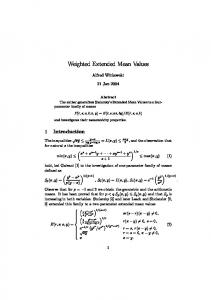
The generalized weighted mean values with two parameters are defined; their basic properties and monotonicities are investigated. Keywords: weighted mean values; monotonicity; basic property; two parameters; Tchebycheff ’s integral inequality; absolutely monotonic function

1. Introduction The subject of mean values is extensive (see, for example, Beckenbach & Bellman 1961; Hardy et al . 1952): a survey of some recent developments can be found in Kuang (1993), Mitrinovi´c (1970) and Mitrinovi´c et al . (1993). Mean values are related to the mean-value theorem for derivatives and integrals, which is the bridge between the local and global properties of functions. Inequalities of mean values form the basis of the theory of analytic inequalities: they have explicit geometric meanings (Qi 1998a). The simplest ‘classical’ means are defined as follows: the arithmetic mean, or average, A(x, y) = 12 (x + y); the geometric mean or mean proportional, G(x, y) = √ xy; and the harmonic mean, H = G2 /A. They have been generalized, refined and extended to many different applications. The root mean square (RMS) is defined as older mean, as Mr (x, y) = ((xr + y r )/2)1/r , N = 12 (G + A), and the power mean, or H¨ r 6= 0, M0 (x, y) = G(x, y). In this paper, the variables x and y are positive. Further evolution led to definitions of other types of means, including: multivariable means with (x1 , . . . , xn ) replacing (x, y); abstracted means Mϕ = ϕ−1 ( 12 (ϕ(x) + ϕ(y))) which reduce to Mr when ϕ(x) = xr ; weighted means given by (1 − α)x + αy and x1−α y α , 0 6 α 6 1; and Lehmer means Lp (x, y) = (xp + y p )/(xp−1 + y p−1 ), p > 0, which reduce to the anti-harmonic mean L2 (x, y) = (x2 + y 2 )/(x + y). Along with the means Mr there are more extended means of particular interest. P´ olya & Szeg¨o (1951) defined the logarithmic mean L by L = L(x, y) =

x−y , ln x − ln y

(1.1)

for x > 0, y > 0, x 6= y and L(x, x) = x. † This paper is dedicated to my dear father, Shu-Gong Qi. Proc. R. Soc. Lond. A (1998) 454, 2723–2732 Printed in Great Britain

2723

c 1998 The Royal Society

TEX Paper

2724

F. Qi

Galvani (1927) considered the extended logarithmic means 1/(p−1)  p y − xp Sp (x, y) = , x 6= y, p 6= 0, 1; p(y − x)

(1.2)

and Sp (x, x) = x; which is reduced to S0 (x, y) = L(x, y), and to the identric mean or the exponential mean I(x, y): S1 (x, y) = I(x, y) = e−1 (xx /y y )1/(x−y) ,

x 6= y;

(1.3)

and S1 (x, x) = I(x, x) = x. The symmetric mean Qp (x, y) is also defined by Qp (x, y) = 12 (xr y s + xs y r ), (1.4) √ √ 1 1 where r = 2 (1 + p), s = 2 (1 − p), p > 0. Alzer (1987) and Yang & Cao (1989) generalized L(x, y) to the one-parameter means  p(y p+1 − xp+1 )  Jp (x, y) = , x 6= y, p 6= 0, −1,    (p + 1)(y p − xp ) (1.5) 2  J0 (x, y) = L(x, y), J−1 (x, y) = G /L,    Jp (x, x) = x. Here, J1/2 (x, y) = h(x, y) is called the Heron mean and J2 (x, y) the centroidal mean. Chen & Shu (1988) introduced the extended Heron means hn (x, y) by hn (x, y) =

1 x1+1/n − y 1+1/n , n + 1 x1/n − y 1/n

(1.6)

and they verified that hn is a decreasing sequence. Stolarsky (1975) defined a two-parameter family of extended means E(r, s; x, y) as follows:   s 1/(s−r) r y − xs   E(r, s; x, y) = , rs(r − s)(x − y) 6= 0,    s y r − xr    r r 1/r E(r, 0; x, y) = E(0, r; x, y) = Lr (x, y) = (L(x , y )) , r(x − y) 6= 0,  (1.7)   E(r, r; x, y) = Ir (x, y) = (I(xr , y r ))1/r , x − y 6= 0,     E(0, 0; x, y) = G(x, y), x 6= y,    E(r, s; x, x) = x, x = y. Stolarsky (1975) also showed that E can be extended to be continuous on the domain {(r, s; x, y) : r, s ∈ R, x, y > 0}. Leach & Sholander (1978, 1983) and P´ ales (1988) investigated the basic properties, monotonicity and comparision of E. A function similar to E that involves a transformation of values of (r, s) was given by Cisbani (1938) and Tobey (1967). Toader (1988, 1989) considered the general means 1/(r−s)  fr (x, y) , (1.8) Mr,s (x, y) = Crs gs (x, y) Proc. R. Soc. Lond. A (1998)

Generalized weighted mean values with two parameters

2725

where fr and gs are homogeneous functions of degree r and s, respectively, and Crs = limt→1 (gs (1, t)/fr (1, t)). The weighted mean of order r of the function f on [a, b] with the weight p is defined (Mitrinovi´c 1970) as  Z 1/r b   r  p(x)f (x) dx       a  r 6= 0,   ,  Z b       p(x) dx  a (1.9) M [r] (f ; p; a, b) =  Z b     p(x) ln f (x) dx      exp  a Z  , r = 0,   b      p(x) dx a

where f and p are defined to be positive and integrable functions on the closed interval [a, b]. The author also researched the mean values (Qi & Xu 1997, 1998; Qi 1998b; Qi & Luo 1998) and the extended means E (Qi 1998a; Qi & Xu 1998) by a simpler method. It is easy to see that the particular means above are special cases of means introduced by Tobey (1967). The study of these means has a rich literature; for details see Carlson (1972), Kuang (1993), Leach & Sholander (1978, 1983), Lin (1974), Mitrinovi´c (1970), Mitrinovi´c et al . (1993) and P´ ales (1988). In this paper, we will define the generalized weighted mean values Mp,f (r, s; x, y) with two parameters r and s, and investigate their basic properties and monotonicities. It is necessary to point out that study of Mp,f (r, s; x, y) is not only interesting but important, both because most of the two variable means, extended mean values and some weighted means are special cases of Mp,f , and because it is challenging to study a function whose formulation is so indeterminate.

2. Definitions and basic properties Definition 2.1. Let x, y, r, s ∈ R, and p(u) 6≡ 0 be a non-negative and integrable function and f (u) a positive and integrable function on the interval between x and y. The generalized mean values, with weight p(u) and two parameters r and s, are defined by Z y 1/(s−r) s p(u)f (u) du  x   , (r − s)(x − y) 6= 0, (2.1) Mp,f (r, s; x, y) =  Z y  r p(u)f (u) du x Z y  r p(u)f (u) ln f (u) du  x   , r(x − y) 6= 0, Z y (2.2) Mp,f (r, r; x, y) = exp    r p(u)f (u) du x

Proc. R. Soc. Lond. A (1998)

2726

F. Qi Z

y

r

1/r

p(u)f (u) du   , r(x − y) 6= 0, y  p(u) du x Z  y p(u) ln f (u) du  x   , x − y 6= 0, Z y Mp,f (0, 0; x, y) = exp    p(u) du  Mp,f (r, 0; x, y) =  

xZ

Mp,f (r, s; x, x) = f (x).

(2.3)

(2.4)

x

For our own convenience, we write Mp,f (r, s; x, y) = Mp,f (r, s) = Mp,f (x, y) = Mp,f , shifting notation to suit the context. Theorem 2.2. Mp,f (r, s; x, y) is continuous on the domain {(r, s; x, y) : x, y, r, s ∈ R}. Proof . This is obvious.



Lemma 2.3. Suppose that f (t) and g(t) > 0 are integrable on [a, b] and the ratio f (t)/g(t) has finitely many removable discontinuity points. There then exists at least one point θ ∈ (a, b) such that Z b f (t) dt f (t) a . (2.5) = lim Z b t→θ g(t) g(t) dt a

We call lemma 2.3 the revised Cauchy mean-value theorem in integral form. Proof . Since f (t)/g(t) has finitely many removable discontinuity points, without loss of generality, suppose it is continuous on [a, b]. Furthermore, using g(t) > 0, from the mean-value theorem for integrals, there exists at least one point θ ∈ (a, b) satisfying  Z b Z Z b f (θ) b f (t) g(t) dt = f (t) dt = g(t) dt. g(t) g(θ) a a a Lemma 2.3 follows.



Theorem 2.4. Mp,f (r, s; x, y) have the following properties: m 6 Mp,f (r, s; x, y) 6 M, Mp,f (r, s; x, y) = Mp,f (r, s; y, x) = Mp,f (s, r; x, y), s−r s−t t−r (r, s) = Mp,f (t, s)Mp,f (r, t), Mp,f where m = inf f (u), M = sup f (u). Proof . They are deduced from the revised Cauchy mean-value theorem in integral form and standard arguments.  Proc. R. Soc. Lond. A (1998)

Generalized weighted mean values with two parameters

2727

3. Monotonicities Lemma 3.1. Let g, h : [a, b] → R be integrable functions, either both increasing or both decreasing. Furthermore, let q : [a, b] → [0, +∞) be an integrable function. Then Z b Z b Z b Z b q(u)g(u) du q(u)h(u) du 6 q(u) du q(u)g(u)h(u) du. (3.1) a

a

a

a

If one of the functions of g or h is non-increasing and the other is non-decreasing, then the inequality (3.1) reverses. Inequality (3.1) is called the Tchebycheff integral inequality (Beckenbach & Bellman 1961; Kuang 1993; Mitrinovi´c 1970; Mitrinovi´c et al . 1993). Ry Proposition 3.2. Let ϕ(t) = x p(u)f t (u) du, where p(u) is a non-negative and continuous function and f (u) is a positive and continuous function on the interval between x and y. If f (u) is monotonic, for k, i, j ∈ N, ϕ(2(i+k)+1) (t)ϕ(2(j+k)+1) (t) 6 ϕ(2k) (t)ϕ(2(i+j+k+1)) (t)

(3.2)

and the ratio ϕ(2(j+k)+1) (t)/ϕ(2k) (t) is increasing. Proof . Taking into account continuity of f (u) which allows us to interchange the derivative and integral, calculating directly results in Z y (n) ϕ (t) = p(u)f t (u)(ln f (u))n du. (3.3) x

Inequality (3.2) is a special case of the Tchebycheff integral inequality applied to the functions q(u) = p(u)f t (u)(ln f (u))2k , g(u) = (ln f (u))2i+1 and h(u) = (ln f (u))2j+1 for i, j, k ∈ N, t ∈ R and u ∈ [x, y]. Using inequality (3.2), simple calculations give  (2(j+k)+1) 0 ϕ(2(j+k+1)) (t)ϕ(2j) (t) − ϕ(2(j+k)+1) (t)ϕ(2j+1) (t) (t) ϕ = > 0.
2 ϕ(2j) (t) ϕ(2j) (t) The desired result follows.



Theorem 3.3. Let p(u) 6≡ 0 be a non-negative and continuous function, f (u) a positive, monotonic and continuous function. Then Mp,f (r, s) increases with both r and s. Proof . First, suppose s = 0. Note that by (2.3) and the definition of ϕ(t), 1/r  ϕ(r) Mp,f (r, 0) = . ϕ(0) We deduce that 1 d (ln Mp,f (r, 0)) = 2 dr r



 ϕ(r) ϕ0 (r) r − ln . ϕ(r) ϕ(0)

By the mean-value theorem and proposition 3.2, it follows that ln Proc. R. Soc. Lond. A (1998)

ϕ(r) ϕ0 (θ) ϕ0 (r) = r< r, ϕ(0) ϕ(θ) ϕ(r)

2728

F. Qi

where θ is between 0 and r. Hence, d(ln Mp,f (r, 0))/dr > 0, so Mp,f (r, 0) increases with r. It is easy to see that Mp,f (r, r; x, y) is increasing in r, from proposition 3.2. For (r − s)(x − y) 6= 0, similar arguments to those above yield   0 ϕ(s) 1 ∂ ϕ (s) (ln Mp,f (r, s)) = (s − r) − ln ∂s (s − r)2 ϕ(s) ϕ(r)   0 ϕ0 (γ) 1 ϕ (s) (s − r) − (s − r) > 0, = (s − r)2 ϕ(s) ϕ(γ) where γ is between r and s. Thus, Mp,f (r, s) is increasing in both r and s, since  Mp,f (r, s) = Mp,f (s, r). Thus the proof of theorem 3.3 is complete. Theorem 3.4. Let p(u) 6≡ 0 be a non-negative continuous function, and f (u) a positive increasing (or decreasing, resp.) continuous function. Then Mp,f (x, y) increases (or decreases, resp.) with respect to either x or y. Proof . Straightforward ∂(ln Mp,f (0, 0; x, y)) = ∂y r (r, 0; x, y)) ∂(Mp,f = ∂y ∂ ln(Mp,f (r, r; x, y)) = ∂y

s−r ∂(Mp,f (r, s; x, y))

∂y

∂ ∂t

Z

y

x

calculation leads to   Z y Z y p(y) (ln f (y)) p(u) du − p(u) ln f (u) du , ϕ2 (0; x, y) x x   Z y Z y p(y) r r (f (y)) p(u) du − p(u)f (u) du , ϕ2 (0; x, y) x x  Z y p(y)f r (y) (ln f (y)) p(u)f r (u) du ϕ2 (r; x, y) x  Z y r p(u)f (u) ln f (u) du , −

p(y)f r+s (y) = 2 ϕ (r; x, y)

p(u)f t (u) du/f t (y)



Z

x

y

x

p(u)f r (u) du/f r (y)  Z y p(u)f s (u) du/f s (y) , −

1 = t f (y)

Z

x

y

x

p(u)f t (u) ln f (u) du  Z y p(u)f t (u) du . − ln f (y) x

From these we conclude that, if f (u) increases (or decreases, resp.),   s−r (r, s; x, y)) ∂(Mp,f = sgn(s − r), (sgn(r − s), resp.), sgn ∂y   r (r, 0; x, y)) ∂(Mp,f sgn = sgn r, (sgn(−r), resp.), ∂y ∂ ln(Mp,f (r, r; x, y)) > 0, (6 0, resp.), ∂y ∂ ln(Mp,f (0, 0; x, y)) > 0, (6 0, resp.). ∂y The desired statements follow. Proc. R. Soc. Lond. A (1998)



Generalized weighted mean values with two parameters

2729

Theorem 3.5. Let p1 (u) 6≡ 0 and p2 (u) 6≡ 0 be non-negative and integrable functions on the interval between x and y, f (u) a positive and integrable function, the ratio p1 (u)/p2 (u) an integrable function, and p1 (u)/p2 (u) and f (u) either both increasing or both decreasing. Then Mp1 ,f (r, s; x, y) > Mp2 ,f (r, s; x, y).

(3.4)

If one of the functions of f (u) or p1 (u)/p2 (u) is non-increasing and the other nondecreasing, then inequality (3.4) is reversed. Proof . Substitution of q(u) = f s (u)p2 (u), g(u) = f r−s (u) and h(u) = p1 (u)/p2 (u) into (3.1) and the standard arguments produce inequality (3.4). This completes the proof of theorem 3.5.  Theorem 3.6. Let p(u) 6≡ 0 be a non-negative and integrable function, and f1 (u) and f2 (u) positive and integrable functions on the interval between x and y. If the ratio f1 (u)/f2 (u) and f2 (u) are integrable and both increasing or both decreasing, then Mp,f1 (r, s; x, y) > Mp,f2 (r, s; x, y)

(3.5)

holds for r, s > 0 or r > 0 > s, and f1 (u)/f2 (u) > 1. The inequality (3.5) is reversed for r, s 6 0 or s > 0 > r, and f1 (u)/f2 (u) 6 1. If one of the functions of f2 (u) or f1 (u)/f2 (u) is non-increasing and the other nondecreasing, then inequality (3.5) is valid for r, s > 0 or s > 0 > r, and f1 (u)/f2 (u) > 1; the inequality (3.5) reverses for r, s > 0 or r > 0 > s, and f1 (u)/f2 (u) 6 1. Proof . The inequality (3.1) applied to q(u) =

p(u)f2r (u),

g(u) =



f1 (u) f2 (u)

r ,

h(u) = f2s−r (u)

and the standard arguments yield theorem 3.6.



4. Applications and miscellanea As concrete applications, we have the following. Proposition 4.1. For special cases of p(u) and f (u), we have the following. (i) Let p(u) ≡ 1, f (u) ≡ u and x, y > 0, then  y 1/(y−x) y −1 Mp,f (0, 0; x, y) = e , (exponential mean), xx 1/r  1 y r+1 − xr+1 , (GLM), Mp,f (r, 0; x, y) = r+1 y−x  yr 1/(yr −xr ) y −1/r Mp,f (r − 1, r − 1; x, y) = e , (identric means), xxr  s 1/(s−r) r y − xs , (extended means), Mp,f (r − 1, s − 1; x, y) = s y r − xr are all increasing with both r and s, or with both x and y. GLM denotes the generalized logarithmic means. Proc. R. Soc. Lond. A (1998)

2730

F. Qi

(ii) Let p(u) = f 0 (u), f (u) be positive and monotonic, then   f (y) 1/[f (y)−f (x)] −1 [f (y)] , Mp,f (0, 0; x, y) = e [f (x)]f (x) 1/r  1 f r+1 (y) − f r+1 (x) , Mp,f (r, 0; x, y) = r+1 f (y) − f (x) r   r f r (y) 1/[f (y)−f (x)] −1/r [f (y)] , Mp,f (r − 1, r − 1; x, y) = e [f (x)]f r (x) 1/(s−r)  s r f (y) − f s (x) , Mp,f (r − 1, s − 1; x, y) = s f r (y) − f r (x) are increasing with both r and s, and have the same monotonicity as f (u) in both x and y. Proposition 4.2. Suppose that f (u) is positive and has derivatives of all orders on the interval [a, b]. Define ψ(t) by  ψ(t) = (f t (b) − f t (a))/t, t 6= 0, (4.1) ψ(0) = ln f (b) − ln f (a), and Un (t, s) as U0 (t, s) = st ,

t

∂Un (t, s) − (n + 1)Un (t, s) = Un+1 (t, s), ∂t

(4.2)

for n ∈ N, s ∈ [a, b]. Then ψ (n) (t) =

Un (t, f (b)) − Un (t, f (a)) , tn+1

∂Un (t, s) = tn+1 (ln s)n st−1 . ∂s

Proof . By (4.2) and direct computation, we find   d (n) d Un (t, f (b)) − Un (t; f (a)) (n+1) ψ (t) = (ψ (t)) = dt dt tn+1 t∂Un (t, f (b))/∂t − (n + 1)Un (t, f (b)) = tn+2 t∂Un (t, f (a))/∂t − (n + 1)Un (t, f (a)) − tn+2 Un+1 (t; f (b)) − Un+1 (t; f (a)) = . tn+2 By the mathematical induction on n, (4.3) is valid. By differentiating (4.2) with respect to s, we obtain ∂ 2 Un ∂Un ∂Un+1 =t − (n + 1) ∂s ∂t∂s ∂s ∂(∂Un /∂s) ∂Un =t − (n + 1) . ∂t ∂s Proc. R. Soc. Lond. A (1998)

(4.3) (4.4)

Generalized weighted mean values with two parameters

2731

Thus, by mathematical induction on n, equation (4.4) is verified. Also, by integrating (4.4) on both sides over the interval [a, b] and using the formulae Z b ψ(t) = f t−1 (u)f 0 (u) du, (4.5) a

ψ (n) (t) =

Z

a

b

f t−1 (u)f 0 (u)[ln f (u)]n du,

we deduce (4.3) easily. This completes the proof of proposition 4.2.

(4.6) 

Definition 4.3. A function f (t) is said to be absolutely monotonic on (a, b) if it has derivatives of all orders and f (k) (t) > 0, t ∈ (a, b), k ∈ N. Definition 4.4. A function f (t) is said to be completely monotonic on (a, b) if it has derivatives of all orders and (−1)k f (k) (t) > 0, t ∈ (a, b), k ∈ N. Definition 4.5. A function f (t) is said to be absolutely convex on (a, b) if it has derivatives of all orders and f (2k) (t) > 0, t ∈ (a, b), k ∈ N. Definition 4.6. A function f (t) is said to be regularly monotonic if it and its derivatives of all orders have constant sign (+ or −; not all the same) on (a, b). From (4.5), (4.6) and definitions 4.3–4.6, the following is deduced directly. Proposition 4.7. If f (u) > 1, f 0 (u) > 0, then the function ψ(t) = [f t (b) − f t (a)]/t, ψ(0) = ln f (b) − ln f (a)

for t 6= 0,

is absolutely and regularly monotonic on the interval (−∞, +∞). If 0 < f (u) 6 1 and f 0 (u) > 0, then ψ(t) is completely and regularly monotonic on (−∞, +∞). Moreover, ψ(t) is absolutely convex on (−∞, +∞). Remark 4.8. The properties and inequalities of absolutely (completely or regularly) monotonic functions and absolutely convex functions have been reviewed (Widder 1941; Mitrinovi´c 1970; Mitrinovi´c et al . 1993). The author was supported in part by NSF grant no. 974050400 of Henan Province, People’s Republic of China. The author is also indebted to the referees for their many helpful comments and for many valuable additions to the list of references.

References Alzer, H. 1987 On Stolarsky’s mean value family. Int. J. Math. Educat. Sci. Tech. 20(1), 186–189. Beckenbach, E. F. & Bellman, R. 1961 Inequalities. Berlin: Springer. Carlson, B. C. 1972 The logarithmic mean. Am. Math. Monthly 79, 615–618. Cisbani, R. 1938 Contributi alla teoria delle medie I. Metron 13(2), 23–34. Chen, J. & Shu, H. 1988 Refinements of Ostle–Terwilliger’s inequality. Shuxue Tongxun, no. 3, pp. 7–8. (In Chinese.) Galvani, L. 1927 Dei limiti a cui tendono alcune media. Boll. Un. Mat. Ital. 6, 173–179. Hardy, G. H., Littlewood, J. E. & P´ olya, G. 1952 Inequalities, 2nd edn. Cambridge University Press. Proc. R. Soc. Lond. A (1998)

2732

F. Qi

Kuang, J. 1993 Applied inequalities, 2nd edn. Changsha: Hunan Education Press. (In Chinese.) Leach, E. & Sholander, M. 1978 Extended mean values. Am. Math. Monthly 85, 84–90. Leach, E. & Sholander, M. 1983 Extended mean values. II. J. Math. Analyt. Appl. 92, 207–223. Lin, T.-P. 1974 The power mean and the logarithmic mean. Am. Math. Monthly 81, 879–883. Mitrinovi´c, D. S. 1970 Analytic inequalities. Berlin: Springer. Mitrinovi´c, D. S., Pe˘cari´c, J. E. & Fink, A. M. 1993 Classical and new inequalities in analysis. Dordrecht: Kluwer. P´ ales, Z. 1988 Inequalities for differences of powers. J. Math. Analyt. Appl. 131, 271–281. P´ olya, G. & Szeg¨ o, G. 1951 Isoperimetric inequalities in mathematical physics. Princeton University Press. Qi, F. 1998a Refinements and extensions of an inequality. Math. Informatics Q. (In the press.) Qi, F. 1998b On a two-parameter family of nonhomogeneous mean values. Tamkang J. Math. 29(2). Qi, F. & Luo, Q. 1998 A simple proof of monotonicity for extended mean values. J. Math. Analyt. Appl. (In the press.) Qi, F. & Xu, S. 1997 Refinements and extensions of an inequality. II. J. Math. Analyt. Appl. 211, 616–620. Qi, F. & Xu, S. 1998 The function (bx − ax )/x: inequalities and properties. Proc. Am. Math. Soc. (In the press.) Stolarsky, K. B. 1975 Generalizations of the logarithmic mean. Math. Mag. 48, 87–92. Toader, Gh. 1988 Mean value theorems and means. In 1st Conf. Appl. Math. Mech. Cluj-Napoca. Toader, Gh. 1989 A generalization of geometric (or) harmonic means. ‘Babes-Bolyai’ Univ. Fac. Math. Phys. Res. Sem. Math. Analysis, no. 2, pp. 21–28. Tobey, M. D. 1967 A two-parameter homogeneous mean value. Proc. Am. Math. Soc. 18, 9–14. Widder, D. V. 1941 The Laplace transform. Princeton University Press. Yang, R. & Cao, D. 1989 Generalizations of the logarithmic mean. J. Ningbo Univ. 2(2), 105–108.

Proc. R. Soc. Lond. A (1998)