IEEE TRANSACTIONS ON INSTRUMENTATION AND MEASUREMENT, VOL. 52, NO. 4, AUGUST 2003
1061
Generating Data With Prescribed Power Spectral Density Piet M. T. Broersen and Stijn de Waele
Abstract—Data generation is straightforward if the parameters of a time series model define the prescribed spectral density or covariance function. Otherwise, a time series model has to be determined. An arbitrary prescribed spectral density will be approximated by a finite number of equidistant samples in the frequency domain. This approximation becomes accurate by taking more and more samples. Those samples can be inversely Fourier transformed into a covariance function of finite length. The covariance in turn is used to compute a long autoregressive (AR) model with the Yule–Walker relations. Data can be generated with this long AR model. The long AR model can also be used to estimate time series models of different types to search for a parsimonious model that attains the required accuracy with less parameters. It is possible to derive objective rules to choose a preferred type with a minimal order for the generating time series model. That order will generally depend on the number of observations to be generated. The quality criterion for the generating time series model is that the spectrum estimated from the generated number of observations cannot be distinguished from the prescribed spectrum. noise, ARMA process, linear filtering, order Index Terms—1 selection, spectral analysis, time series models.
I. INTRODUCTION
T
HE ACCURACY of many experiments is limited by the presence of measurement noise in the observations. It will certainly be a problem in sensitive satellite measurement data [1]. Often, a good characterization of the noise spectrum is known from previous experiments or from a detailed physical description of the sensor and its environment. In such circumstances, it is possible to test the signal processing sequence in advance by using a noise realization of a stochastic process that has the known spectral density. The purpose may be to verify that the proposed signal processing allows for the desired accuracy. One specific application is the new gravity field and ocean circulation explorer mission, to be launched in 2006 [1]. This mission aims at the development of an improved model of the earth’s gravity field. The presence of colored observation noise in a huge number of observations leads to a difficult numerical regression problem, demanding a weighted least squares solution. The weighting matrix is the inverse of the extremely large covariance matrix of the noise. The power spectral density of the colored noise is concentrated in the low frequency part. A time series description of the known noise spectral density gives the possibility to generate noise realizations. The same time series model can be used to design an inverse filter for Manuscript received June 15, 2002; revised April 16, 2003. The authors are with the Department of Applied Physics, Delft University of Technology, Delft, The Netherlands (e-mail:
[email protected]). Digital Object Identifier 10.1109/TIM.2003.814824
the colored noise; for real-time implementation, it is important that the filter has a low order. The filtered noise becomes uncorrelated, which is an important advantage in the remaining regression problem [1]. Other examples for the generation of data emerge in turbulence, where the spectrum is proportional and in other physical problems, e.g., with noise. to Time series modeling is a parametric description of spectral densities. The three model types that can be used for time series models are autoregressive (AR), moving average (MA), and combined ARMA models. All stationary stochastic processes can be characterized by AR or by MA models of infinite order [2]. AR models are more suitable for spectral peaks; MA models are better for valleys. In practice, most processes can be de) processes scribed adequately by AR( ), MA( ), or ARMA( of finite orders and/or [3]. Generating stationary data for a given ARMA process requires some care. Using zeros or any arbitrary values as initial conditions, generated signals become stationary after the duration of the impulse response. Unfortunately, the impulse response is only finite for a MA process. It is infinitely long for AR and ARMA processes. Therefore, this primitive method of data generation without care for initial conditions can only be exact for MA processes. It is at best an approximation for AR or ARMA processes. A better method is found by separating the generation into an AR and a MA part. Consider the joint probability density function of a finite number of AR observations with a prescribed correlation function. Data can be generated that obey that prescribed AR correlation. A realization of the ARMA process is obtained by filtering AR data with the MA polynomial. So far, it has been assumed that the spectral requirements are already formulated as a time series model. However, prescriptions for data can also be given in terms of correlation functions or power spectral densities. In principle, observations can be considered as a single period of a multisine signal, that can be disgiven the prescribed spectral density at maximally . Multisine crete frequencies signals are particularly appropriate as input signals for system identification at a limited number of frequencies, but not for apnoise. The discrete spectrum would require plications like a new signal specification for each value of , at different frequencies. It would only have the desired spectral properties for sample sizes that are multiples of , if care is taken with the transients of the initial conditions. Therefore, the treatment of these types of prescriptions for data also preferably uses time series models, which produce stationary stochastic data with a continuous spectral density that can be generated for different values of with the same model. A solution has been given to
0018-9456/03$17.00 © 2003 IEEE
1062
IEEE TRANSACTIONS ON INSTRUMENTATION AND MEASUREMENT, VOL. 52, NO. 4, AUGUST 2003
fit an AR, MA, or an ARMA model to a finite number of sampled spectral values [4]. It uses the inverse Fourier transform of the spectrum as the desired covariance function. An AR model of high order is calculated then from those covariances with the Yule–Walker relations [2]. The AR model is also a basis to compute other time series models. Models can often be simplified by using the long AR model as input for a reduced statistics analysis [4]. This paper describes the joint probability density function (pdf) of an arbitrary number of observations of an AR( ) process. That is the basis for the generation of data. Prescribed spectral densities can be based on estimated or on exact knowledge. It is shown that order selection criteria can be adapted to the reliability or the accuracy of the spectral prescriptions. Furthermore, it is shown that an adequate generating process for the prescribed spectral density may depend on the number of observations to be generated. II. ARMA MODELS An ARMA(
) process is defined as [2]
spectrum. The ME is a scaled transformation of the expectation of the squared error of prediction PE (4) The model error is asymptotically equal to distortion SD, defined as
(5) where the denotes an approximating spectrum. In this way, the ME can also be defined for spectral densities that are not given by time series models. The expectation of ME is for unbiased models independent of and of the variance of the signal. Only true and estimated parameter values are required to compute the ME with (4). The asymptotical expectation of the ME of unbi) models that contain at ased efficiently estimated ARMA( least all truly nonzero parameters is equal to the number of estimated parameters. III. PROBABILITY DENSITY OF AR PROCESS
(1) represents a series of independent, identically diswhere tributed, zero mean white noise observations. The process is 0 and MA for 0. The ARMA process can purely AR for also be written with polynomials of AR and of MA parameters as (2) and . Models may have estimated polynomials of arbitrary orders, not necessarily equal to the true and . Processes and models are stationary if the poles, the estimated , are inside the unit circle; they are invertible if the roots of , are inside the unit circle. The spectral zeros, the roots of density is given by [2]
times the spectral
The normal distribution of a variable with mean is given by ance
and vari-
(6) observations , where The joint pdf of mally distributed vector stochastic variable
with
is a jointly nor(7)
with
(8) is given by
(3) This shows that the parameters of a time series model, together with the variance of the exciting white noise, determine the spectral density. The covariance function is the inverse integral Fourier transform of (3). It can be approximated by an inverse . However, it is discrete Fourier transform of a sampled also possible to obtain an exact covariance function for a given ) process by direct computations in the time domain ARMA( [2]. Therefore, the parameters of a time series model are a good representation for the characteristics of a process, exact in both the time and in the frequency domain. ) models with polynoThe quality of estimated ARMA( mials indicated by is measured with the model error ME [5]. This measure can be used in simulations where an omniscient ) parameters experimenter knows the true process ARMA( that generated the observations. Likewise, it can be used to evaluate the difference between a prescribed spectral density, expressed as an ARMA process and the approximating ARMA
(9) This is a general expression that can be applied to AR, MA, in or ARMA processes by expressing the Toeplitz matrix the parameters. It is often preferred in the literature and it has computational advantages to use as much as possible the white noise innovations with diagonal covariance function in the probability density and likelihood functions [2]. The observations are then considered as filtered innovations. The probability density function of observations of an AR( ) process with poly, with normally distributed zero mean innovations nomial can also be written as a conditional product of the last observations, given the first
(10)
BROERSEN AND DE WAELE: GENERATING DATA WITH PRESCRIBED POWER SPECTRAL DENSITY
The first part of the right-hand side for the last tions is given by [2, p. 347]
observa-
1063
The variance of the AR( ) process is given by (18)
(11)
The recursive variance relation for intermediate AR orders can be expressed with increasing or decreasing index, which gives
The second part describing the first observations is also known [2, p. 350]. However, a recursive form of that expression is a better starting point for the generation of data. By using conditional densities, it follows that:
(19)
Now, the conditional density (17) becomes (12) Generally, for all observations , with
(13) With those intermediate results for , (12) can be written as (20) (14) Elements of the Levinson–Durbin algorithm [6] can be used to evaluate this expression. This algorithm recursively computes from the AR correlaparameter sets of increasing order tion function, as well as variance expressions. The last parameter of an AR model of order is always equal to the reflection coefficient . The algorithm starts with
(15) denotes the covariance of the AR( ) process at lag where . The recursion for is given by [7, p. 169]
The substitution of (20) in (14) and that result together with (11) in (10) is merely an exercise with as result sums of products. However, as all ingredients for the probability density function are given, the derivation is sufficient to be used in generating data for an AR( ) process. IV. DATA GENERATION Data generation is strictly separated in MA and AR generation. For ARMA processes, it is essential that the AR part is used first, because the derivation of Section III used white noise as input, e.g., in (11). Remind that the covariances in (16) are covariances belonging to the AR polynomial only. The principle is for ARMA processes given by
(21) which together combines to the result of (2) (22) AR
Data
is At the final stage of the recursion, the polynomial in (2). The polynomial is the best equal to , or the best linear combination of linear predictor of order previous observations to predict the next observation . Hence, the conditional probability density of , conditional on previous observations has as expectation with the variance . Using this in the conditional expectations (13) gives with (6)
observations with the probaThe purpose is to generate like in (10). The first bility density function observation has the only requirement that it has expectation or . That is found with a random zero and variance number generator with normal or Gaussian density and the prescribed variance. The second observation follows from (15) and (17) as a normally distributed random variable with mean and variance . The third observation uses (16) and and variance . The first obser(17) with mean vations are generated in this way. According to (11), all further observations can be generated with the regime
(17)
(23)
(16)
1064
IEEE TRANSACTIONS ON INSTRUMENTATION AND MEASUREMENT, VOL. 52, NO. 4, AUGUST 2003
This is a filter procedure with a Gaussian random white noise signal as input signal and the first observations as initial conditions. For AR processes, the initial observations and the filter results with (23) are together the observations. MA
or ARMA(
integration interval , a correlation function as proximated from discrete values
can be ap-
) Data
for the second equation in For MA data, the input signal (21) is a Gaussian white noise . For ARMA processes, the input to the MA filter will be the output of the AR filter (23). are computed with The data (24) The first data require negative input index. Therefore, to generate MA or ARMA observations with this method, the input long. The first points of the filter sequence has to be output are disregarded. V. FROM SPECTRUM TO ARMA MODEL Data are always generated with the time series model (1), using white noise of a random generator as input. Therefore, the prescribed spectral density will at the end be defined by the parameters of an ARMA model. If the parameters are already given as characterization for the desired spectral density, they can be used immediately. However, the prescribed spectrum can also be given as an exact continuous function . Without loss of generality, the sampling time is taken to be 1. The first step is to determine an approximation for the cois the inverse variance function. The covariance function integral Fourier transform of the continuous function
(25) may be infinite. By defining ) periodic The length of with period 2 , the integral in (25) can also be taken from 0 to 2 . As in (25) is continuous, the usual discrete time inverse Fourier computer transformations can only be approximations , unless specific assumptions can be made about the infor terpolated values between the discrete frequency values that are used in the computation. Different covariance functions . can belong to the same finite sampled discrete version of A unique finite covariance may be found by considering the process as a MA process [6], which has nonzero values for only a finite range of shifts . Also, considering a finite part of the covariance function as a Fourier series gives an unique inter[2, p. 578] with the FFT polation in a continuous function algorithm. However, the true covariance function of an AR or an ARMA process is infinitely wide, albeit that it will be damping in (25) by a summaout. Approximating the integral of tion is equivalent with sampling in the frequency domain. This causes the equivalent of aliasing of the covariance function, in the time domain. Therefore, some care in the covariance calculation with inverse Fourier transform is required. Taking the as representative for an mid-range value of the integrand
(26) , this summation is almost equal to the usual sumFor small has the limiting value 1 mation result in (26) because is obtained if many equidisfor small . A small value for are used. The derivation of (26) for tant points is preferred above the usual inverse FFT if only a few samples are used in the inverse transformation. It is also of a given possible that the prescribed spectral density is specified for only a small number of frequencies. The integration in (26) defines and are explicitly what is transformed. However, if given, it is always more accurate to use the standard time series formulae for the calculation of the covariance function for a finite number of shifts [2]. Integration with (26) or any other approximation of the integral can only provide exact results for the covariance function if the true process is MA. For one-sided prescribed spectra defined for between 0 at intervals , with and , the first step is to sample . The samples are samples for made to a symmetric spectrum by adding the in reversed order. Taking gives a convenient length for the FFT. After the inverse Fourier transform of ) points the elongated sampled spectrum, the first , ( describe the desired covariance function. should be chosen high enough, such that the values of the covariance are effectively zero for lags beyond . If that turns out to be impossible for a prescribed spectrum because the covariance function is too elongated, should be chosen at least as high as the number of observations that has to be generated. The larger , the better the estimated covariance. This is an operational advice for the length and it should always be validated that the correlation . The first lags of the is negligible beyond , or that covariance function are transformed to an AR( ) model with is exact, the Yule–Walker relations [6]. If the prescribed taking and greater will generally give a better approximation; the improvement may be small. If the true process is a finite MA( ) process, no problems arise as long as the correlation length is taken greater than . All other processes have an infinite long covariance function that generally damps out quickly. The question is if some value of the AR order, less than or , can be considered high enough for an approximation of sufficient accuracy for data generation. It may be advantageous to have a low-order process to generate data. It is still more important to design a low order filter to undo the coloring of some given spectral density to whiten the noise will finally become notice[1]. Any distortion of the true able if more and more data are generated. Therefore, the minidepends on the number of observations mally required order
BROERSEN AND DE WAELE: GENERATING DATA WITH PRESCRIBED POWER SPECTRAL DENSITY
that has to be generated. A natural choice is to allow distortions that are much smaller than the expected statistical uncertainty if the generated data are analyzed. The distortion can be quantified as the bias of the truncated model in the ME measure (4) or in the spectral distortion (5). If the bias contribution of the truncation is smaller than the variance contribution to the ME of estimating a single parameter, the higher order parameters can be omitted without the possibility that the omission can be detected from generated observations. This is no tight boundary but it is a sensible compromise. This gives an allowed ME of 1 for the truncated AR( ) model with respect to the true AR( ) process for a given . With (4), this gives (27) This is the lowest order
, for which the AR(
) model gives
(28) In practice, the AR( ) process in (28) is replaced by the finite chosen at least so high that the order AR( ) process, with ) model has a difference between the AR( ) and the AR( ME difference smaller than say 0.1 for the given . This can be verified in practice and can be chosen higher until this conand dition is met. Simulations will indicate that orders are often much smaller than . It is possible to use the AR( ) model as input for a reduced statistics algorithm [4] that computes AR, MA, and ARMA models of various orders. Moreover, it will select the model type and the model order that are closest to the given AR( ) process. Furthermore, the MA model with ) model with lowest the lowest order and the ARMA( order can be found that have a ME value less than 1 with respect to the AR( ) model, for a given value of . In this way, or or , can be the minimum number of parameters, determined that is required to meet the accuracy demands. If the would be a finite order MA( ) or ARMA( ) true process process, this finite order can easily be detected with the reduced statistics estimator. If this MA or ARMA model requires less parameters than the AR( ) model described before, it may be worthwhile to use the most parsimonious time series model to generate or to filter data. However, it should be realized that the MA and ARMA models have long transients in inverse filtering. Using lower order models will give a less accurate approximation of the prescribed spectrum. It is also possible to define a prescribed spectrum with an estimated periodogram, instead of with a continuous function . In those cases, special care is required, because estimated obserperiodograms contain a lot of spurious details. If vations are transformed with the FFT and the absolute values are squared, the resulting function is the raw periodogram, say . The inverse Fourier transform of should be the covariance function, but it is an aliased version which has as expectation [2] (29)
1065
with . Using tapers and windows will cause more distortions of the covariance. The use of periodograms cannot be advised. Periodograms as a spectral prescription can be of the same accuracy as some very high-order estimated AR model, if the triangular bias in (29) is negligible [3]. However, a much better solution exists. If one wants to use measured data as prototype for the spectrum, it is advised to estimate the time series model for those data with ARMAsel [8]. This automatic computer program finds the best spectral time series model for given data with robust algorithms and criteria, which select only statistically significant details. is not Another possibility is that the information in exact, at least not for all frequencies. For colored satellite noise, the spectral density at some discrete, not equidistant, is frequencies has been given and the continuous function determined with interpolation [1]. The proposed method to deal with those circumstances is largely the same as dealing with , but with a completely different critical value for the exact ME. Variation of the interpolation methods and spline solutions produces different continuous spectra, different covariances, and, hence, different time series models. The difference between those interpolation solutions can be expressed in the ME (4) for a given value of as the number of data to be generated. If no information about the best interpolation is available, all solutions are equally well obeying the prescriptions. The largest difference found in the ME between the different interpolation results can be used as a critical ME value, instead of the critical that was derived before for a given exact true value ME . In this way, lower order models may become accurate enough if the prescription is less precise. The practical criterion for data generation is always: generate observations with a time series spectrum that cannot be distinguished from the true given spectrum. It might be possible that the model is good for the generation of observations, but the difference can, perhaps, be seen if the same model was used to generate 100 or more observations. Therefore, the generating model may depend on . VI. SIMULATIONS To show the possibilities of the data generation, it is applied to an example where broken exponents determine the desired spectral shape. It is some prototype spectrum for turbulence data. The spectrum consists of two declining slopes after a constant at the lowest frequencies. The first slope descends at a rate of from 0.01 and the second slope of starts at 0.1 (30) and Fig. 1 shows no visible difference between the true the AR(1000) approximation. The ME difference between the , truncated AR(500) and the AR(1000) model is . According to the rules which is less than 0.1 for developed in Section V, data can be generated with sufficient accuracy if the ME of the truncated model is less than 1. Table I presents those orders. It is clear that the data generation can be carried out with a very high accuracy. Taking much lower
1066
IEEE TRANSACTIONS ON INSTRUMENTATION AND MEASUREMENT, VOL. 52, NO. 4, AUGUST 2003
Fig. 1. Turbulence prototype spectrum and approximating AR(1000) model for L = 2 0 .
Fig. 2. 1=f prototype spectrum and approximating AR(4096) model for L = K = 4096.
TABLE I LOWEST ALLOWED TRUNCATED AR ORDER M WITH THE ME LESS THAN 1 FOR THE GENERATION OF N TURBULENCE OBSERVATIONS, AS A FUNCTION OF N ; L = 2 AND K = 1000
TABLE II LOWEST ALLOWED TRUNCATED AR ORDER M WITH THE ME LESS THAN 1 FOR THE GENERATION OF N FROM 100 TO 100 000 OBSERVATIONS, AS A FUNCTION OF L AND K , FOR 1=f AS PRESCRIBED SPECTRAL DENSITY. N IS THE NUMBER FOR WHICH THE AR(K ) AND THE AR(K=2) MODEL HAVE 0.1 AS THEIR ME DIFFERENCE
values for , the length of the inverse Fourier transform, has hardly any influence on the minimum order . The values for obtained with and 500 are equal to those in Table I, except the last one that becomes 141. This demonstrates that this turbulence covariance function is already damped out sufficiently at lag 500. The sampling distance in the frequency domain hardly influences the estimated covariance function and of the AR model is greater the AR parameters if the length than 500. spectrum An interesting spectral density in physics is the in Fig. 2. The normalized true spectrum and an approximation are shown. Both have the same sum of the total power in the , it is difficult or normalization. Due to the singularity at even impossible to generate data that obey this spectrum. The length of the approximating covariance function is strongly influenced by the value of . Particularly, the approximating finite and the choice for , devalue of the spectrum taken for termining the smallest nonzero sampled frequency at or , have an enormous impact on the length of the correlation. On the other hand, it is impossible to recognize or shape from observations at frequencies to verify the . This is visible in Fig. 2 because the aplower than say proximating spectrum becomes inaccurate for less than say spectrum, a choice 0.0001 . In approximating this true , because the true value of the spectrum had to be made for becomes infinite and leads to numerical problems. Therefore, some extrapolation from the first two nonzero sampled values have been used. Those are at the frequencies for and . A parabola through the spectrum of those two points,
with the additional demand that the derivative of the spectrum equals 0 yields: . at spectrum. Table II gives some results for the prescribed depends much more on than on because The value for the length of the approximating covariance function depends strongly on . If is chosen long enough, the actual value of has almost no influence. The necessary AR orders are much higher than for the turbulence example. Despite that, the accuracy at very low frequencies is still not good. The accuracy of AR models of different orders is shown in Fig. 3. The low order models in Fig. 3 are still reasonable for higher frequencies. , AR(100) is reasonable for AR(10) is reasonable for , and AR(1000) is reasonable for . The full length AR(4096) model is shown in Fig. 2. This demonstrates that it is possible to find a satisfactory time series model . However, in cases with for any , by selecting at least , the required minimum model order a singularity at is rather high. It can be advised to always compare visually the truncated AR spectra with the prescription, like in Fig. 3. The in Table II is a minimum; using the full truncation value of length gives always a better approximation. The first example shows that smooth spectral shapes can be modeled easily with time series models. The second example
BROERSEN AND DE WAELE: GENERATING DATA WITH PRESCRIBED POWER SPECTRAL DENSITY
1067
order for the generating process gives ARMAsel results that are closer to the spectrum for a larger part of the frequency range. VII. CONCLUSION
Fig. 3. 1=f prototype spectrum and three AR approximations for L = K = 4096.
Data with a prescribed spectral density can be generated in a simple way with time series models. The first step is to determine a finite-order AR model that has a spectrum close enough to the prescribed spectrum. Several tools are available to facilitate the search for a parsimonious time series model of other types. Use of higher orders always improves the accuracy, unless the spectral prescriptions were specified as a finite-order time series model. By using an exact description of the probability density funcautoregressive observations as a product of condition of tional probabilities, it is possible to efficiently generate autoregressive data. The generation of MA or ARMA data is solved with a simple filter operation. REFERENCES [1] R. Klees, P. Ditmar, and P. M. T. Broersen, “How to handle colored observation noise in large least-squares problems?,” J. Geodesy, vol. 76, pp. 629–640, 2003. [2] M. B. Priestley, Spectral Analysis and Time Series. London, U.K.: Academic, 1981. [3] P. M. T. Broersen, “Automatic spectral analysis with time series models,” IEEE Trans. Instrum. Meas., vol. 51, pp. 211–216, Apr. 2002. [4] P. M. T. Broersen and S. de Waele, “Selection of order and type of time series models from reduced statistics,” in Proc. IEEE/IMTC Conf., Anchorage, AK, May 2002, pp. 1309–1314. [5] P. M. T. Broersen, “The quality of models for ARMA processes,” IEEE Trans. Signal Processing, vol. 46, pp. 1749–1752, June 1998. [6] S. M. Kay and S. L. Marple, “Spectrum analysis—A modern perspective,” Proc. IEEE, vol. 69, pp. 1380–1419, Nov. 1981. [7] P. J. Brockwell and R. A. Davis, Time Series: Theory and Methods. New York: Springer-Verlag, 1987. [8] P. M. T. Broersen. ARMASA Toolbox. [Online]. Available: http://www.tn.tudelft.nl/mmr/downloads.
Piet M. T. Broersen was born in Zijdewind, The Netherlands, in 1944. He received the M.Sc. degree in applied physics and the Ph.D. degree from the Delft University of Technology (DUT), Delft, The Netherlands, in 1968 and 1976, respectively. He is currently with the Department of Applied Physics, DUT. His main research interest is in automatic identification on statistical grounds. He found a solution for the selection of order and type of time series models for stochastic processes and the application to spectral analysis, model building, and fea-
Fig. 4. 1=f prototype spectrum, the AR(63) approximation for L = K = and the ARMAsel spectrum selected from 1000 observations that had been generated with the AR(63) process.
2
deals with the problem that the estimated covariance will always depend on the arbitrary length . That determines the sampling distance in the frequency domain and, therefore, the lowest nonzero frequency, which is taken into account in the transforgives some guarmation of the true spectrum. Taking antee that the differences between the generating process and the prescribed spectrum are not noticeable from observations. This is demonstrated in Fig. 4 where the ARMA(5,4) spectrum is shown that was selected with the ARMAsel algorithm [8] from 1000 observations that were generated with the AR(63) . The resulting ARMAsel specmodel obtained with , reasonable for and trum is good for poor for still lower frequencies. It closely follows the AR(63) spectrum that generated the observations. Taking a higher AR
ture extraction.
Stijn de Waele was born in Eindhoven, The Netherlands, in 1973. He received the M.Sc. degree in applied physics and the Ph.D. degree, with a thesis entitled “Automatic model inference from finite time observations of stationary stochastic processes,” from the Delft University of Technology, Delft, The Netherlands, in 1998 and 2003, respectively. Currently, he is a Research Scientist at Philips Research Laboratories, Eindhoven, The Netherlands, where he works in the field of digital video compression.