Generating Meaningful Test Databases

I NAUGURAL - D ISSERTATION

zur Erlangung der Doktorwürde der Naturwissenschaftlich-Mathematischen Gesamtfakultät der Ruprecht-Karls-Universität Heidelberg

vorgelegt von M.Sc. Carsten Binnig aus Buchen

Tag der mündlichen Prüfung: 15.4.2008

G ENERATING M EANINGFUL T EST DATABASES

Gutachter:

Prof. Dr. Donald Kossmann Prof. Dr. Barbara Paech

Abstract Testing is one of the most time-consuming and cost-intensive tasks in software development projects today. A recent report of the NIST [RTI02] estimated the costs for the economy of the Unites States of America caused by software errors in the year 2000 to range from $22.2 to $59.5 billion. Consequently, in the past few years, many techniques and tools have been developed to reduce the high testing costs. Many of these techniques and tools are devoted to automate various testing tasks (e.g., test case generation, test case execution, and test result checking). However, almost no research work has been carried out to automate the testing of database applications (e.g., an E-Shop application) and relational database management systems (DBMSs). The testing of a database application and of a DBMS requires different solutions because the application logic of a database application or of a DBMS strongly depends on the contents of the database (i.e., the database state). Consequently, when testing database applications or DBMSs new problems arise compared to traditional software testing. This thesis focuses on a specific problem: the test database generation. The test database generation is a crucial task in the functional testing of a database application and in the testing of a DBMS (also called test object further on). In order to test a certain behavior of the test object, we need to generate one or more test databases which are adequate for a given set of test cases. Currently, a number of academic and commercial test database generation tools are available. However, most of these generators are general-purpose solutions which create the test databases independently from the test cases that are to be executed on the test object. Hence, the generated test databases often do not comprise the necessary data characteristics to enable the execution of all test cases. In this thesis we present two innovative techniques (Reverse Query Processing and Symbolic Query Processing), which tackle this problem for different applications (i.e, the functional testing of database applications and DBMSs). The idea is to let the user specify the constraints on the test database individually for each test case in an explicit way. These constraints are then used directly to generate one or more test databases which exactly meet the needs of the test cases that are to be executed on the test object.

i

Zusammenfassung In heutigen Softwareentwicklungsprojekten ist das Testen eine der kosten- und zeitintensivsten Tätigkeiten. Wie ein aktueller Bericht des NIST [RTI02] zeigt, verursachten Softwarefehler in den USA im Jahr 2000 zwischen 22, 2 und 59, 5 Milliarden Dollar an Kosten. Demzufolge wurden in den letzten Jahren verschiedene Methoden und Werkzeuge entwickelt, um diese hohen Kosten zu reduzieren. Viele dieser Werkzeuge dienen dazu die verschiedenen Testaufgaben (z.B. das Erzeugen von Testfällen, die Ausführung von Testfällen und das Überprüfen der Testergebnisse) zu automatisieren. Jedoch existieren fast keine Forschungsarbeiten zur Testautomatisierung von Datenbankanwendungen (wie z.B. eines E-Shops) oder von relationalen Datenbankmanagementsystemen (DBMS). Hierzu sind neue Lösungen erforderlich, da das Verhalten der zu testenden Anwendung stark vom Inhalt der Datenbank abhängig ist. Folglich ergeben sich für den Test von Datenbankanwendungen oder von Datenbankmanagementsystemen neue Probleme und Herausforderungen im Vergleich zum traditionellen Testen von Anwendungen ohne Datenbank. Die vorliegende Arbeit diskutiert ein bestimmtes Problem aus diesem Umfeld: Die Generierung von Testdatenbanken. Die Generierung von Testdatenbanken ist eine entscheidende Tätigkeit für den erfolgreichen Test einer Datenbankanwendung oder eines Datenbankmanagementsystems (im weiteren Verlauf auch Testobjekt genannt). Um eine bestimmte Funktionalität des Testobjekts zu testen, müssen die Daten in den Testdatenbanken bestimmte Charakteristika aufweisen. Zur Erzeugung einer Testdatenbank existieren verschiedene Forschungsprototypen wie auch kommerzielle Datenbankgeneratoren. Jedoch sind die existierenden Datenbankgeneratoren meist Universallösungen, welche die Testdatenbanken unabhängig von den auszuführenden Testfällen erzeugen. Demzufolge weisen die generierten Testdatenbanken meist nicht die notwendigen Datencharakteristika auf, die zur Ausführung einer bestimmten Menge von Testfällen notwendig sind. Die vorliegende Doktorarbeit stellt zwei innovative Ansätze vor (Reverse Query Processing und Symbolic Query Processing), die dieses Problem für unterschiedliche Anwendungen (d.h. für das funktionale Testen von Datenbankanwendungen und Datenbankmanagementsystemen) lösen. Die generelle Idee beider Ansätze ist, dass der Benutzer explizit für jeden Testfall die notwendigen Bedingungen an die Testdaten formulieren kann. Diese Bedingungen werden dann dazu genutzt, um eine oder mehrere Testdatenbanken zu generieren, die die gewünschten Datencharakteristika aufweisen, welche zur Ausführung der Testfälle notwendig sind.

ii

Acknowledgments First of all, I would like to express my deep gratitude to Professor Donald Kossmann who supervised and guided my research work in the last three years together with Professor Barbara Paech. From the very beginning Professor Donald Kossmann put trust in me and motivated me to strive for the highest goals. While I was struggling with some hard research problems, he encouraged me to continue and he showed me that I need to step back and see the big picture. Moreover, he spent much time with me to discuss the pros and cons of doing a PhD even before I started to work with him. Furthermore, I would also like to thank Professor Barbara Paech. Without her help it would not have been possible for me to conduct my research work at the University of Heidelberg. She always put trust in me and gave me all the support that I needed to follow my research interests. Moreover, there are a lot of other people who supported me during the last three years: In the first place, I would like to thank Eric Lo. Together with him, I spent a vast amount of time behind closed doors in productive discussions about our crazy research ideas. We constantly motivated each other which finally made our both dreams come true. Alike, I would also like to thank José A. Blakeley who supported me in applying my research ideas to an industrial environment at Microsoft Corporation in Redmond. Moreover, he introduced me to many other nice and supportive colleagues who assisted me in realizing my research ideas for Microsoft in a very short time. Furthermore, life would not have been as much fun without all the other colleagues and students at the University of Heidelberg and at the ETH Zurich. Especially, I would like to mention my colleague Peter Fischer in Zurich who helped me in many technical and administrative issues in a completely unselfish way. Alike, I would like to thank two students, Nico Leidecker and Daniil Nekrassov, who helped me in implementing some of my concepts. Finally, I would like to thank my wife Daniela and my family for their enduring support while I was working on my research ideas in the past few years.

iii

Contents

I Preliminaries

1

1 Introduction

2

1.1

Motivation . . . . . . . . . . . . . . . . . . . . . . . . . . . . . . . . . . . . . . . . . . .

2

1.2

Contributions and Overview . . . . . . . . . . . . . . . . . . . . . . . . . . . . . . . . .

5

2 Background

7

2.1

Software Testing: Overview and Definitions . . . . . . . . . . . . . . . . . . . . . . . . .

7

2.2

State of the Art . . . . . . . . . . . . . . . . . . . . . . . . . . . . . . . . . . . . . . . .

9

2.2.1

Testing Database Applications and DBMSs . . . . . . . . . . . . . . . . . . . . .

9

2.2.2

Generating Test Databases . . . . . . . . . . . . . . . . . . . . . . . . . . . . . .

14

2.2.3

Resume . . . . . . . . . . . . . . . . . . . . . . . . . . . . . . . . . . . . . . . .

16

II Reverse Query Processing

19

3 Motivating Applications

20

4 RQP Overview

23

4.1

Problem Statement and Decidability . . . . . . . . . . . . . . . . . . . . . . . . . . . . .

24

4.2

RQP Architecture . . . . . . . . . . . . . . . . . . . . . . . . . . . . . . . . . . . . . . .

25

4.3

RQP Example . . . . . . . . . . . . . . . . . . . . . . . . . . . . . . . . . . . . . . . . .

28

5 Reverse Relational Algebra

29

5.1

Reverse Projection . . . . . . . . . . . . . . . . . . . . . . . . . . . . . . . . . . . . . .

30

5.2

Reverse Selection . . . . . . . . . . . . . . . . . . . . . . . . . . . . . . . . . . . . . . .

30

5.3

Reverse Aggregation . . . . . . . . . . . . . . . . . . . . . . . . . . . . . . . . . . . . .

31

5.4

Reverse Join, Cartesian Product . . . . . . . . . . . . . . . . . . . . . . . . . . . . . . .

31

5.5

Reverse Union . . . . . . . . . . . . . . . . . . . . . . . . . . . . . . . . . . . . . . . . .

31

5.6

Reverse Minus . . . . . . . . . . . . . . . . . . . . . . . . . . . . . . . . . . . . . . . .

32

5.7

Reverse Rename . . . . . . . . . . . . . . . . . . . . . . . . . . . . . . . . . . . . . . .

32

v

CONTENTS

6 Bottom-up Query Annotation

33

6.1

Leaf initialization . . . . . . . . . . . . . . . . . . . . . . . . . . . . . . . . . . . . . . .

35

6.2

Reverse Join . . . . . . . . . . . . . . . . . . . . . . . . . . . . . . . . . . . . . . . . . .

36

6.3


39

6.4


43

6.5


43

6.6

Reverse Union . . . . . . . . . . . . . . . . . . . . . . . . . . . . . . . . . . . . . . . . .

45

6.7

Reverse Minus . . . . . . . . . . . . . . . . . . . . . . . . . . . . . . . . . . . . . . . .

46

6.8

Reverse Rename . . . . . . . . . . . . . . . . . . . . . . . . . . . . . . . . . . . . . . .

46

6.9

Annotation of Nested Queries . . . . . . . . . . . . . . . . . . . . . . . . . . . . . . . .

47

7 Top-down Data Instantiation

48

7.1

Iterator Model . . . . . . . . . . . . . . . . . . . . . . . . . . . . . . . . . . . . . . . . .

49

7.2


50

7.3


53

7.4

Reverse Join . . . . . . . . . . . . . . . . . . . . . . . . . . . . . . . . . . . . . . . . . .

53

7.5


54

7.6

Reverse Union . . . . . . . . . . . . . . . . . . . . . . . . . . . . . . . . . . . . . . . . .

54

7.7

Reverse Minus . . . . . . . . . . . . . . . . . . . . . . . . . . . . . . . . . . . . . . . .

55

7.8

Reverse Rename . . . . . . . . . . . . . . . . . . . . . . . . . . . . . . . . . . . . . . .

55

7.9

Special Cases . . . . . . . . . . . . . . . . . . . . . . . . . . . . . . . . . . . . . . . . .

55

7.9.1

Reverse Join . . . . . . . . . . . . . . . . . . . . . . . . . . . . . . . . . . . . .

55

7.9.2

Reverse Projection and Reverse Aggregation . . . . . . . . . . . . . . . . . . . .

59

7.9.3

Reverse Union . . . . . . . . . . . . . . . . . . . . . . . . . . . . . . . . . . . .

63

7.10 Processing Nested Queries . . . . . . . . . . . . . . . . . . . . . . . . . . . . . . . . . .

63

7.11 Optimization of Data Instantiation . . . . . . . . . . . . . . . . . . . . . . . . . . . . . .

65

8 Reverse Query Optimization

69

8.1

Optimizer Design . . . . . . . . . . . . . . . . . . . . . . . . . . . . . . . . . . . . . . .

70

8.2

Query Unnesting . . . . . . . . . . . . . . . . . . . . . . . . . . . . . . . . . . . . . . .

70

8.3

Other Rewrites . . . . . . . . . . . . . . . . . . . . . . . . . . . . . . . . . . . . . . . .

72

9 Experiments

73

9.1

Experimental Environment . . . . . . . . . . . . . . . . . . . . . . . . . . . . . . . . . .

73

9.2

Size of Generated Databases . . . . . . . . . . . . . . . . . . . . . . . . . . . . . . . . .

74

9.3

Running Time (SF=0.1) . . . . . . . . . . . . . . . . . . . . . . . . . . . . . . . . . . . .

75

9.4

Running Time: Varying SF . . . . . . . . . . . . . . . . . . . . . . . . . . . . . . . . . .

76

10 Related Work

77

vi

CONTENTS

III Applications of Reverse Query Processing

79

11 Functional Testing of OLTP Applications

81

11.1 MRQP Overview . . . . . . . . . . . . . . . . . . . . . . . . . . . . . . . . . . . . . . .

85

11.1.1 Problem Statement and Decidability . . . . . . . . . . . . . . . . . . . . . . . . .

85

11.1.2 MRQP Restrictions . . . . . . . . . . . . . . . . . . . . . . . . . . . . . . . . . .

85

11.1.3 MRQP Solution . . . . . . . . . . . . . . . . . . . . . . . . . . . . . . . . . . . .

90

11.2 The DB Generation Language MSQL . . . . . . . . . . . . . . . . . . . . . . . . . . . .

91

11.2.1 Query Classes and Algebra . . . . . . . . . . . . . . . . . . . . . . . . . . . . . .

92

11.2.2 Adjust Operations for Query Refinements . . . . . . . . . . . . . . . . . . . . . .

94

11.2.3 MSQL Example . . . . . . . . . . . . . . . . . . . . . . . . . . . . . . . . . . .

96

11.2.4 Queries and Result Variables . . . . . . . . . . . . . . . . . . . . . . . . . . . . .

97

11.2.5 Query Rewrites . . . . . . . . . . . . . . . . . . . . . . . . . . . . . . . . . . . .

99

11.3 Reducing the Test Databases . . . . . . . . . . . . . . . . . . . . . . . . . . . . . . . . . 101 11.4 Related Work . . . . . . . . . . . . . . . . . . . . . . . . . . . . . . . . . . . . . . . . . 103 12 Functional Testing of a Query Language

104

12.1 Functional Testing of SQL . . . . . . . . . . . . . . . . . . . . . . . . . . . . . . . . . . 106 12.1.1 Generating the Expected Query Result . . . . . . . . . . . . . . . . . . . . . . . . 106 12.1.2 Verifying the Actual Query Result . . . . . . . . . . . . . . . . . . . . . . . . . . 107 12.2 The ADO.NET Entity Framework . . . . . . . . . . . . . . . . . . . . . . . . . . . . . . 109 12.3 Reverse Query Processing Entity SQL . . . . . . . . . . . . . . . . . . . . . . . . . . . . 111 12.3.1 Discussion and Overview . . . . . . . . . . . . . . . . . . . . . . . . . . . . . . . 111 12.3.2 Extended Nested Relational Data Model . . . . . . . . . . . . . . . . . . . . . . . 113 12.3.3 Reverse Nested Relational Algebra . . . . . . . . . . . . . . . . . . . . . . . . . 115 12.4 Related Work . . . . . . . . . . . . . . . . . . . . . . . . . . . . . . . . . . . . . . . . . 119 13 Other Applications

120

IV Symbolic Query Processing

123

14 Motivating Applications

124

15 SQP Overview

129

15.1 Problem Statement and Decidability . . . . . . . . . . . . . . . . . . . . . . . . . . . . . 129 15.2 SQP Architecture . . . . . . . . . . . . . . . . . . . . . . . . . . . . . . . . . . . . . . . 130 15.2.1 Query Analyzer . . . . . . . . . . . . . . . . . . . . . . . . . . . . . . . . . . . . 131 15.2.2 Symbolic Query Engine and Database . . . . . . . . . . . . . . . . . . . . . . . . 133 15.2.3 Data Instantiator . . . . . . . . . . . . . . . . . . . . . . . . . . . . . . . . . . . 134 15.3 Supported Symbolic Operations . . . . . . . . . . . . . . . . . . . . . . . . . . . . . . . 134 16 Query Analyzer

136

vii

CONTENTS

17 Symbolic Query Engine 139 17.1 Symbolic Data Model . . . . . . . . . . . . . . . . . . . . . . . . . . . . . . . . . . . . . 139 17.1.1 Definitions . . . . . . . . . . . . . . . . . . . . . . . . . . . . . . . . . . . . . . 139 17.1.2 Data Storage . . . . . . . . . . . . . . . . . . . . . . . . . . . . . . . . . . . . . 140 17.2 Symbolic Operations . . . . . . . . . . . . . . . . . . . . . . . . . . . . . . . . . . . . . 141 17.2.1 Table Operator . . . . . . . . . . . . . . . . . . . . . . . . . . . . . . . . . . . . 141 17.2.2 Selection Operator . . . . . . . . . . . . . . . . . . . . . . . . . . . . . . . . . . 143 17.2.3 Equi-Join Operator . . . . . . . . . . . . . . . . . . . . . . . . . . . . . . . . . . 149 17.2.4 Aggregation Operator . . . . . . . . . . . . . . . . . . . . . . . . . . . . . . . . 153 17.2.5 Projection Operator . . . . . . . . . . . . . . . . . . . . . . . . . . . . . . . . . . 161 17.2.6 Union Operator . . . . . . . . . . . . . . . . . . . . . . . . . . . . . . . . . . . . 161 17.2.7 Minus Operator . . . . . . . . . . . . . . . . . . . . . . . . . . . . . . . . . . . . 162 17.2.8 Intersect Operator . . . . . . . . . . . . . . . . . . . . . . . . . . . . . . . . . . . 162 17.2.9 Processing Nested Queries . . . . . . . . . . . . . . . . . . . . . . . . . . . . . . 163 18 Data Instantiator

164

19 Semi-Automatic DBMS Testing

167

19.1 The Framework . . . . . . . . . . . . . . . . . . . . . . . . . . . . . . . . . . . . . . . . 170 19.2 Test Case Generation . . . . . . . . . . . . . . . . . . . . . . . . . . . . . . . . . . . . . 170 20 Experiments 174 20.1 Efficiency of Symbolic Operations . . . . . . . . . . . . . . . . . . . . . . . . . . . . . . 174 20.2 Scalability of QAGen . . . . . . . . . . . . . . . . . . . . . . . . . . . . . . . . . . . . . 176 20.3 Effectiveness of the Semi-Automatic Testing Framework . . . . . . . . . . . . . . . . . . 176 21 Related Work

181

V Summary

183

22 Conclusions and Future Work

184

A Analysis of the Approximate Overweight Subset-Sum Problem

187

A.1 Correctness . . . . . . . . . . . . . . . . . . . . . . . . . . . . . . . . . . . . . . . . . . 187 A.2 Time and Space Complexities . . . . . . . . . . . . . . . . . . . . . . . . . . . . . . . . 189 B Complexity of the Group Assignment Problem

viii

190

Part I

Preliminaries

1

Chapter

1

Introduction I think and think for months and years, ninety-nine times, the conclusion is false. The hundredth time I am right. – Albert Einstein, 1879-1955 –

1.1 Motivation Testing is one of the most time-consuming and cost-intensive tasks in the software development projects today. A recent report of the NIST [RTI02] estimated the costs for the economy of the Unites States of America caused by software errors in the year 2000 to range from $22.2 to $59.5 billion (or about 0.6 percent of the gross domestic product). While one half of these costs result from error avoidance and mitigation activities of the users, the other half is borne by software developers due to inadequate testing techniques and tools. Another study [Erl00] in the E-Business sector stated that roughly 90 percent of the total software costs are spent on system maintenance and evolution which includes development costs to identify and correct software defects. Consequently, in the past few years many techniques and tools have been developed by industry and academia to reduce the costs caused by software errors and the time spent for testing activities. Many of these techniques and tools are devoted to automate various testing tasks (e.g., the test case generation, the test case execution, and the test result checking). According to [Bal06], the worldwide market for Automated Software Quality Tools was about $948 million in 2005 and will be higher than $1 billion in 2006, and $1.8 billion in 2010. However, almost no research work has been carried out to automate the testing of database applications and relational database management systems (DBMSs). The testing of a database application

2

1.1 MOTIVATION

or of a DBMS needs different solutions because the application logic of a database application or of a DBMS strongly depends on the content of the database (database state)1 . Consequently, when testing database applications or DBMSs, new problems and opportunities arise compared to traditional software testing. For example, [HKL07] showed that traditional test case scheduling techniques in the test execution phase do not work optimally for database applications. Moreover, [HKL07] illustrated that specialized scheduling strategies can reduce the total running time of the test execution phase dramatically. This thesis focuses on another specific problem: the test database generation. The test database generation is a crucial task in the functional testing of a database application or a DBMS (called test object further on). In order to test a certain behavior of the test object, we need to generate a database state that satisfies certain data characteristics. A simple example is a login function of an E-Shop like Amazon which rejects users to log in after having tried to log in more than three times with an incorrect password. In order to test that function thoroughly, the test database should comprise a user who has not yet tried to log in wrongly more than three times to test the positive case where the user is not rejected. Moreover, the test database should also comprise another user who has already entered an incorrect password more than three times, to test the negative case where the user is rejected by the login function. Another example is the testing of a DBMS. Most of the functionality of a DBMS strongly depends on the data characteristics of the stored data; e.g., the optimizer of a query execution engine chooses the physical execution plan depending on the data characteristics of the underlying database and the data characteristics of the intermediate query results. If we want to test the functionality of the query optimizer thoroughly, it is necessary to vary the data characteristics which are used to calculate the costs of the alternative query plans. Currently, a number of academic and commercial tools are available which generate test databases. These tools can be classified into two categories: either the test database is extracted from a live database, or a synthetic test database is generated according to a given database schema. The existing tools which extract the test database from a live database suffer from various problems: One problem is that using a live database may not always be possible, because of data protection regulations; another problem is that a live database often does not comprise all the necessary data characteristics to enable the execution of all interesting test cases (e.g., there is no user in the live database who has tried to log in more than three times with the incorrect password). Consequently, generating a synthetic test database seems to be the panacea to solve these problems. However, existing tools which generate synthetic test databases suffer from the same problem; i.e., the generated test databases do not comprise all the data characteristics necessary to execute a given set of test cases. The reason is that the existing tools are general-purpose solutions which take constraints on the complete database state as input (e.g., table sizes and value distributions 1

In this thesis we use the terms database state, database instance, and test database as synonyms.

3

CHAPTER 1: INTRODUCTION

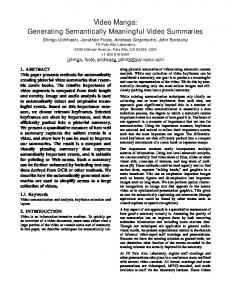
Test Cases

Test Cases

T1

T1 T2

T2

T4 T3

T4 T3

Test Database

Test Database(s) (b) Test Case Aware Database Generation

(a) Random Test Database Generation

Figure 1.1: Test Database Generation Problem

of individual attributes). However, these constraints are not suitable to express the relevant data characteristics necessary to execute each individual test case. Consequently, the test databases are usually generated independently from the needs of the individual test cases. We call these approaches which generate the test database independently from the test cases Random Test Database Generation techniques. Conceptually, this problem is demonstrated in Figure 1.1 (a): This figure shows a test database which is generated independently from a set of given test cases {T1 , T2 , T3 , T4 }. Using this randomly generated test database, only some test cases (e.g., T2 and T3 ) can be executed, while the other test cases (e.g., T1 and T4 ) cannot be executed at all. In order to deal with this problem in practice, the generated test databases are often modified manually in order to fit to the needs of all test cases. As a result, the maintenance of a test database becomes hard because a manual modification of the test database for a new or a modified test case often corrupts the test database for other test cases that are to be executed on the same test database. In this thesis we present two innovative techniques which tackle the test database generation problem in a different way by enabling a Test Case Aware Database Generation; i.e., one or more test databases are generated which exactly fit to the needs of the test cases that are to be executed on the test object (as shown in Figure 1.1 (b), the generated test databases enable the execution of all test cases). The main idea of the Test Case Aware Database Generation is to let the user specify constraints on the database state individually for each test case in an explicit way. These constraints are then used directly to generate one or more test databases which exactly satisfy the constraints specified by the test cases that are to be executed on the test object. For example, when testing a database application, it is necessary to formulate constraints on the

4

1.2 CONTRIBUTIONS AND OVERVIEW

values of individual tuples (and not on the complete database state); e.g., to test the login function of the E-Shop application, the tester needs to specify that two different users exist in the test database (i.e., one who is allowed to log in and one who is not allowed to log in). Alike, when testing a DBMS, it is important that the data characteristics of the intermediate query results of a test query, and not only the characteristics of the base tables, can be controlled explicitly in order to test a particular behavior of the DBMS.

1.2 Contributions and Overview The main contributions of this thesis are the formal concepts and prototypical implementations of two new test database generation frameworks (called Reverse Query Processing [BKL06b; BKL06a; BKL07b] and Symbolic Query Processing [BKL07a; BKLO07]) which generate test case aware databases for the functional testing of OLAP applications (e.g., a reporting application) and for the functional testing of DBMS components (e.g., the cardinality estimation component). Both frameworks are extensible and thus not bound to a specific application, even though they are motivated by the particular applications mentioned above. As a further contribution, we discuss two more applications of Reverse Query Processing in detail; i.e., the functional testing of OLTP applications (like an E-Shop) [BKL08] as well as the functional testing of a query language [BKLSB08]. Moreover, we also present the required extensions of RQP to support these two applications. Furthermore, we show how the extensions of RQP for the functional testing of a query language can be used in an industrial environment. Finally, we sketch some other applications of Reverse Query Processing which need additional research. For both frameworks we carried out a set of experiments to analyze the performance and the effectiveness of our prototypical implementations under a variety of workloads. The remainder of the thesis is structured as follows: • In the next chapter, we present the background in software testing and illustrate the state of the art in the testing of database applications and DBMSs as well as the state of the art in test database generation. • In Part II of this thesis, we discuss the first framework which enables a test case aware database generation (called Reverse Query Processing or RQP for short). The main application of RQP is the functional testing of OLAP applications. • In Part III we illustrate two further applications of RQP in detail (i.e., the functional testing of OLTP applications as well as the functional testing of a query language) and discuss the

5

CHAPTER 1: INTRODUCTION

extensions of RQP which are necessary to support these applications. Moreover, we sketch other potential applications of RQP. • Subsequently, in Part IV we describe the second framework which enables a test case aware database generation (called Symbolic Query Processing or SQP for short). SQP is designed to generate test databases for the functional testing of individual DBMS components. • Finally, Part V contains the conclusions (i.e., the current state of this work and its limitations) as well as suggestions for future work (i.e., research problems and potential improvements for a better industrial applicability). A more detailed discussion of the individual contributions and a detailed outline will be given separately for each part.

6

Chapter

2

Background Knowledge is of two kinds. We know a subject ourselves, or we know where we can find information upon it. – Samuel Johnson, 1709-1784 –

2.1 Software Testing: Overview and Definitions Software Testing is the execution of a component or a system using combinations of input and state to reveal defects [Bin99] by verifying the actual output. The component or system under test is called the test object. Depending on the test level the test object is of different granularity: In Unit Testing the test object is usually a method or a class, in Integration Testing the test object is the interface among several units, and in System Testing the test object is a complete integrated application. In software testing the terminology is very often not clear. In this thesis we refer to the terminology defined in [IST06]. Especially, the terms failure, defect, and error are often used as synonyms while a having a different meaning: A failure is the inability of a test object to perform a function within certain limits; i.e., the system or component returns an incorrect output, terminates abnormally, or does not terminate within certain time constraints. A defect is the missing or incorrect code that caused the failure of the test object. An error is the human action that produced a defect (e.g., by coding). Testing can only show the presence of defects in a test object but never their absence. Software testing activities can have different testing objectives: One possible objective is to reveal defects through failures (which is called fault-directed testing). Another objective is to demon-

7

CHAPTER 2: BACKGROUND

strate the conformance of a test object to the required capabilities (which is called conformancedirected testing). A conformance-directed test type is functional testing which checks the conformance of the test object with the specification of the functionality. Another conformance-directed test type is usability testing which checks the conformance of the user interface to some usability guidelines or performance testing which checks the conformance to some time restrictions etc. A test case usually specifies the test object, the inputs that are used to exercise the test object as well as the state of the test object before the test case is executed (called precondition); e.g., external files, contents of the database. Moreover, a test case defines the expected output and the expected state of the test object after the test case execution (called postcondition). The expected output and the postcondition are often called test oracle. A test suite is a set of test cases that are related; e.g., by a common test objective. A test run is the execution of a test suite which comprises a set of test cases. A test case is executed as follows: First, in a set-up phase the precondition is used to the set the state of the test object. Afterwards, the test object is exercised using the given input. Finally, the actual output and the state after the execution of the test case are compared to the expected output and the expected state (postcondition) in order to verify the test results and decide whether a test case passes or not. Executing all possible test cases (which is called exhaustive testing) by using all combinations of input values and preconditions to execute the test object is practically impossible because the number of all combinations of input values and preconditions is usually too huge. For, example assume that we want to test a method that takes ten 8-bit integer values as input. The possible input space would be (28 )10 . If we could execute 1000 test cases per second then it would take approximately 41.210 days which is roughly 38334786263782 years to run all test cases for exhaustive testing. In order to deal with that problem various test design techniques can be used to derive and select the test cases that shall be exercised on a test object. Black-box test design techniques are based on an external view of the test object, and not on its implementation; i.e., black-box test design techniques analyze the external behavior to derive test cases. One example of a black-box test design technique are equivalence classes. Equivalence classes partition the domain of the individual input values into sub-domains for which the behavior of the test object is assumed to be the same. The idea of equivalence classes is that the tester can pick one value out of each class instead using all possible input values. In contrast to black-box test design techniques, white-box test design techniques are based on the internal structure of a test object which can be the result of a source code analysis. One example of a white-box test design technique is control-flow testing which uses the information about the control-flow to execute different code paths of the test object. While white-box test design techniques are more often used for fault-directed testing (e.g., to find a division by zero), black-box test design techniques are more often used for conformance-directed testing (e.g, to check whether the test object behaves as specified or not).

8

2.2 STATE OF THE ART

The coverage of a test suite is measured by a coverage metric. A typical coverage metric for white-box testing is the statement coverage which defines the percentage of executable statements that have been exercised by a test suite. A coverage metric for black-box testing is the equivalence class coverage. The equivalence class coverage is defined as ratio of the number of tested equivalence classes and the number of all equivalence classes; i.e., the metric shows the percentage of equivalence classes that have been exercised by a particular test suite [IST06]. The goal of test automation is to minimize the manual overhead necessary to execute certain test activities; e.g., test case generation, test case execution and test result checking. In most cases test automation can be seen as a system engineering problem to implement a special kind of software which executes the test activity automatically. Test automation has several benefits compared to manual testing. For example, the automation of the test case execution helps to run more test cases in a certain time span and thus to increase the test coverage. Moreover, test automation makes testing repeatable because humans tend to vary the test cases during manual execution. Thus, automating the test case execution is a precondition for effective regression testing while the goal of regression testing is to execute one or more test suites after the test object has changed and compare its behavior before and after the changes.

2.2 State of the Art This section gives an overview of the state of the art related to this thesis: First, we discuss some general problems that arise when testing a database application or a DBMS and show several solutions to these problems. Afterwards, we study the problem of generating test databases in Section 2.2.2 in detail. While some of these approaches deal with a similar problem statement as this thesis (i.e., the generation of test case aware databases), some other approaches discuss orthogonal aspects (i.e., efficient algorithms for generating huge data sets or algorithms for generating various data distributions).

2.2.1

Testing Database Applications and DBMSs

In the past years many techniques and tools have been developed by academia and industry to automate the different testing activities [Bin96]. Surprisingly, relatively little attention has been given to developing systematic techniques to support the individual testing tasks for database applications and DBMSs [Kap04]. In the following, we discuss specific problems and opportunities that arise when testing database applications and DBMSs. Moreover, we briefly illustrate some of the existing work.

9


Test Database Generation:

Before a test suite of a database application or a DBMS can be

executed, it is necessary to create an initial database state that is appropriate for each test case. For example, as mentioned in the introduction, in order to execute a test case of an E-Shop application which executes the login function, different types of users need to be created. Currently, some industrial tools (e.g., [IBM; DTM; dbM]) and research prototypes (e.g., [BC05; SP04; HTW06; NML93; CDF+ 04; MR89; ZXC01; WE06]) are available which generate test databases. However, most of these tools generate the test databases independent from the test cases that are to be executed on the test database. Consequently, in many cases the generated test databases are not appropriate to execute all intended test cases. The reason is that the existing tools are general-purpose solutions which offer only very limited capabilities to constrain the generated test database (i.e., most tools take only the database schema as input and generate random data over that schema). However, these constraints are not adequate to express the needs of the individual test cases which should to be executed on the database application or the DBMS. Consequently, as the test databases are generated independent from the test cases there has also been no work on the evolution of the test database if the test suite changes (e.g., new test cases are added or existing test cases are modified). Currently, the only way to deal with the evolution of a test suite is to regenerate the test database completely. As this thesis focuses on the problem of generating test case aware databases, we present some of the existing tools in more detail separately in the next Section 2.2.2.

Test Case Generation:

In order to generate test cases for database applications and DBMSs,

new test design techniques need to be developed because existing techniques cannot deal with the semantics of database applications and DBMSs. When testing a DBMS, for example, a test case usually comprises one or more SQL queries that are issued against the test database. Traditional test design techniques like equivalence classes are hardly applicable to automatically create test cases (i.e., SQL queries) for DBMS systems and the huge domain of possible SQL queries. Thus, different tools like RAGS [Slu98] and QGEN [PS04] have been developed to quickly generate SQL queries that cover interesting query classes for a given database schema and other input values (e.g., a parse tree, statistical profiles). In order to extend a given test suite with further interesting test cases, [TCdlR07] devises some mutation operators for SQL queries to generate new test queries from a given set of test queries. Another work [BGHS07] (which was used to test the SQL Server 2005) presents a genetic approach to create a set of test queries (i.e., a test suite) for DBMS testing. The initial set of test queries is created randomly; e.g., by using approaches like RAGS and QGEN. Moreover, each time before a test suite is executed, a new test query is generated by mutating the queries of the existing test suite. Afterwards, the queries of test suite and the new query are executed on the DBMS and execution feedback (e.g., query results, query plan, traces that expose internal DBMS

10


state) is collected. Based on the execution feedback a fitness function determines whether a newly created test case will be added to the test suite or not. For example, the fitness function could use existing code coverage metrics to decide whether the new test query increases the coverage of the test suite or not. When testing database applications instead of DBMSs, a test suite should cover test cases that exercise the different execution paths of the application. However, standard test design techniques do not work properly because they do not consider the database state when test cases are created. As a result, the test cases may not cover all interesting execution paths. For example, when testing the login function of an E-Shop application then not all interesting test cases might be created (e.g., to test different users where one user has already tried to log in more than three times with the incorrect password and another user has not). In [yCC99] the authors argue that existing white-box test design techniques generate test cases that do not cover all interesting code paths because the semantics of SQL statements that are embedded in a database application are rarely considered. Thus, the authors suggest to transform the declarative SQL statements into imperative code and then to apply existing white-box test design techniques to create test cases. The objective of the transformation is to include the semantics of the SQL statements into the imperative code so that more test cases are generated to reveal defects that result from different internal database states. For example, a function of an E-Shop application that displays the books of a particular author could use a 2-way join query on authors and books that is embedded in the code to extract the necessary data from the database. In order to test that function, the 2-way join is transformed into a nested loop statement in the application code. Using the transformed code as input, white-box design techniques will generate test cases that cover different database states: one test case could execute the function for an author with no books which means that the nested loop is not executed at all, and another test case could execute that function for an author with n books which means that the nested loop is executed n times. Another drawback of many existing test design techniques is that they create test cases which do not specify the database state before and after the execution of a test case (i.e., as pre- and postconditions). Consequently, the test cases cannot be used to set the database state before the execution and to check the database state after the execution. The work in [RDA04] presents a framework for the black-box testing of database applications called AutoDBT. AutoDBT takes a specification of the user navigation (as a finite state machine), a data specification which defines constraints on the database for each transition in the user navigation, as well as an initial database state as input and generates test cases that can be executed on the given database state. Using the data specification, AutoDBT can track the database changes of each test case (i.e., AutoDBT can calculate a set of pre- and postconditions on the database state).

11


Consequently, AutoDBT can decide whether the precondition of a test case holds (i.e., if the test case can be executed on the current database state) and whether the postcondition is satisfied when the test case was executed (i.e., if the database is in the expected state). For example, for a test case which deletes a given book of an E-Shop, AutoDBT will check (1) if the book exists before the test case is executed and (2) if the book was deleted successfully after the test case was executed.

Coverage metrics: As we discussed in Section 2.1 the coverage of a test suite is measured by a coverage metric. However, existing test coverage metrics cannot deal with the semantics of database applications and DBMSs. In order to tackle that shortcoming, [KS03] proposed a new family of coverage metrics for the white-box testing of database applications which capture the interactions of a database application with a database at multiple levels of granularity (attribute, tuple, relation, database) . The test coverage metric uses the dataflow information that is associated with the different entities in a relational database (i.e., how many percent of the attributes, tuples, or relations are read or updated by a given test suite). The empirical study in [KS03] confirms that a significant number of important database interactions are overlooked by traditional coverage metrics. Another work [CT03] proposed a new coverage metric for testing SQL statements. The idea is to apply an existing coverage metric, the multiple condition coverage [MS77], to SQL statements. This coverage metric analysis if a given predicate is evaluated thoroughly in all possible ways for a given test database. For a SQL query, the metric in [CT03] analysis if the join and selection predicates of a given SQL query are evaluated to true and false for the different tuples in the test database. If a predicate is a complex predicate with conjunctions and disjunctions then the coverage metric analysis each simple predicate. For example, if a SQL query contains the predicate b_aid = a_id ∧ a_name = ‘Knuth‘ then the coverage metric checks if the complete predicate evaluates to true and false for different tuples of the test database and if each simple predicate (b_aid = a_id and a_name = ‘Knuth‘) does so, too. Based on that information the value of the coverage metric is calculated.

Test Case Execution:

When executing test cases for database applications and DBMSs a par-

ticular database state has to be reset before each test case can be executed in order to guarantee a deterministic behavior of the test object. For example, assume that we want to execute a test case T1 of an E-Shop application that lists all books of a particular author (who has written 100 books) and the test cases passes if all 100 books are displayed. However, if another test case T2 (which deletes all books of that author) is executed before test case T1 , then T1 will fail because no books are displayed (i.e., the expected result is different from the actual result). Thus, a trivial solution to avoid this problem is to set the appropriate database state each time before the test case is executed. However, this can take very long if the test database is huge: e.g., it already takes about

12


two minutes to reset a 100MB database [HKK05]. Moreover, traditional execution strategies do not consider that fact when scheduling the test cases for a test run. Consequently, if a test suite should be used for nightly regression tests, then not all test cases might be executed because of the unexpected long running time. Consequently, the authors in [HKL07] devised several scheduling algorithms which try to find an optimal order of the test cases in a test suite with the goal to minimize number of database resets. This work assumes that all test cases of a test suite can use the same database state. Consequently, if no test case of a test suite updates the test database, then the database state has to be reset only once at the beginning of a test run. Thus, the basic idea of the algorithms in [HKL07] is to apply the database reset lazily; i.e., a test case of a test suite is executed without setting the appropriate database state. If the test case execution fails, then the database state is reset and the test case is re-executed. If the test case passes afterwards, then the test case has a conflict with a previously executed test case which updated the database state. Otherwise, the test case detected a failure. During a test run (i.e., the execution of a test suite), the algorithms learn which test cases are possibly conflicting with each other (i.e., which test case might have updated the database state so that another test case fails). As a result, the scheduling algorithms reorder the conflicting test cases of a test suite for the next test run with the goal to reduce the number of necessary database resets. For example, the following test suite is executed in the given order: T = {T1 , T2 , T3 } . Assume that only T3 fails because of a “wrong” database state (which was caused by an update of T1 and/or T2 ). Then for the next test run, the scheduling algorithms would reorder the test suite to avoid the conflict of the test case T3 with test cases T1 and/or T2 . A new order could be T = {T3 , T1 , T2 }.

Test Result Verification/Test Oracle:

When executing a test case on a database application or

a DBMS, the actual test results (actual output and state of the test database) have to be verified in order to decide whether a test case passes or fails. In the regression testing of database applications, the expected output of a test suite is created by executing the test cases on the test object and recording the behavior of the test object [HKK05] (called recording phase). During the recording phase, the test object is expected to work correctly. After modifications of the database application, the test suite is re-executed (called playback phase) and the actual results are compared to the expected (recorded) results. While regression testing needs a running application to create the test oracle, other test techniques derive the expected results from specifications of the test object (e.g., as discussed in [RDA04]). Another idea for verifying the result when testing the query processing engine of a DBMS is illustrated in [Slu98]. In order to verify the actual results of the test queries, the author of [Slu98] propose to execute the test queries on a comparable DBMS which returns the expected results for

13


verification. This idea can be generalized and used for the test result verification of other kinds of test objects (not only DBMSs), too.

2.2.2

Generating Test Databases

In this section we present several test database generation tools. These tools can be classified into two categories: either a synthetic test database is generated or the test database is extracted from a live database.

Synthetic Test Databases: Currently, there are a number of commercial tools available (e.g., [IBM; DTM; dbM]) which generate a random test database over a given database schema. Beside the database schema, some tools also support the input of the table sizes, data repositories and additional constraints used for data instantiation (e.g. statistical distributions, value ranges). Most of the commercial tools are not extensible (e.g., the set of supported data distributions is fixed). Additionally, a number of academic tools are available which generate test databases. Some of them are designed to be extensible in a few aspects. For example, [BC05] tackles the problem that most existing tools support only a fixed set of data distributions. However, in order to thoroughly evaluate new DBMS techniques (e.g., new access methods, histograms, and optimization strategies) varying data distributions need to be generated. Consequently, this work presents a flexible framework to specify and generate test databases using rich data distributions as well as intraand inter-table correlations for a given database schema. The framework is based on composable iterators that generate data values, whereas the set of iterators can be extended by the user. [SP04] presents another test database generation framework (called MUDD) that can also be extended by complex user defined data distributions. MUDD was designed to generate test databases for the TPC-DS benchmark [TPCa] and thus is intended for use in the performance evaluation of DBMS decision support solutions. MUDD also supports varying database schemes. Moreover, [HTW06] also developed a database generator which is also intended to be used in the performance evaluation of DBMS decision support solutions. Again, the user can easily add new data types and distributions. In addition, their tool takes a graph model and some data dependencies as input: The graph model specifies the database schema and thus defines the order how the tables are populated. The data dependencies (e.g., foreign-key constraints) further constrain the database state. A different tool which takes a set of user defined predicates as input to generate the test database is presented in [NML93]. The tool supports a subset of the first-order-logic and thus allows the definition of more complex constraints as the tools discussed before which only take the database schema and some data distributions as input. However, [NML93] showed that their approach to

14


generate a test database which meets a set of arbitrary constraints formulated in first-order-logic does not scale for large test databases and complex constraints. All the tools discussed before generate test databases independent of the test cases that are to be executed on the test object. The tools that we illustrate in the sequel try to tackle this problem by taking some information about the test cases as input (i.e., the application queries of the database application or the test queries that are to be executed on the DBMS). In [CDF+ 04] a set of tools for testing database applications (called AGENDA) is presented. One tool of AGENDA is a database generator which takes a database schema (with integrity constraints), an application query and some sample values as input. The selection predicate of the application query is used to partition the domains of all attributes that participate in the predicate into equivalence classes. For example, if a SQL query defines a filter predicate 10 ≤ b_price ≤ 100 then three partitions are generated for the attribute b_price: ]−∞, 10[, [10, 100], and ]100, ∞[. For other attributes not in the selection predicate, the user can define the equivalence classes manually. The database generator offers different heuristics to guide the test database generation process: one heuristic is to generate boundary values for the specified equivalence classes; another heuristic is to generate NULL values if possible, etc. Another work which also takes a SQL query as input is presented in [MR89]. The goal of this work is to generate a test database for a given relational query (limited to simple select-projectjoin queries) so that the query result is unique for the given test query; i.e., no other non-equivalent query exists that returns the same result for the generated test database. A test database which satisfies this criteria can be used for the testing of a query language; i.e., for such a test database it is easier to decide whether the actual result of a test query is the expected result or not because the expected result can be returned for only one particular test query (i.e., two non-equivalent queries must have different expected results). In [ZXC01] the authors study the generation of test databases for the white-box testing of database applications. The goal of this work is to generate a test database which returns a result that has certain characteristics for a given SQL query in order to execute a particular code path of the application. The tool supports only select-project-join queries as input and the user can specify that the result of such a query should be empty or not and she can also add domain constraints on the result attributes (e.g., all values of the b_price attribute should be greater 0). In order to generate the test database, all the constraints on the query result are translated into a constraint satisfaction problem which can be solved by existing constraint solvers. A similar tool is presented in [WE06]. The only difference to [ZXC01] is that the constraint formula which is used to generate the test database for a given database schema is constructed more systematically; i.e., the SQL query is translated into a relational algebra expression and the query operators transform the constraints on the query result into constraints on the database schema. For example, a projection operator adds the deleted attributes to the constraint formula

15


to let the constraint solver instantiate values for those attributes. Again, only select-project-join queries are supported as input. In contrast to all tools discussed before, [GSE+ 94] focuses on particular problems that arise when huge synthetic databases need to be generated. This work is orthogonal to all tools presented above. In particular, this work discusses how parallelism can be used to get generation speed-up and scale-up and presents algorithms to generate huge data sets that follow various distributions (e.g., uniform, exponential, normal). Moreover, solutions to generate indexes concurrent to the base table are discussed, too. Extracts from Live Databases: Another alternative to generate test databases is to extract the data from a live database. However, extracting data from a live database might be problematic because the use of data from live databases has the potential to expose sensitive data to an unauthorized person. Moreover, a live database may not cover all interesting data characteristics adequate to test a particular behavior of the test object. In [WSWZ05], the authors investigate a method to generate a so called mock database based on some a-priori knowledge about the live database without revealing any confidential information of the live database. The techniques of this work guarantee that the mock database will have almost identical statistics compared to the live database. Consequently, the mock database can be used to evaluate the performance of a database application. A similar approach can be found in [BGB05]. The authors of this work devise a formal framework for database sampling. Their initial motivation was to generate a test database for testing new features of a database application. The framework extracts a test database from a live database that meets the same integrity constraints as the live database and includes all the “data-diversity” found in the live database. The resulting database is expected to better support the development of new features of a database application than a synthetic test database.

2.2.3

Resume

Some approaches for generating test databases that we presented in Section 2.2.2 [CDF+ 04; MR89; ZXC01; WE06] discuss the same problem statement as this thesis; i.e., generating test case aware databases. However, all these approaches fall short in many aspects tackled by this work: • The main drawback of all these approaches is that they generate test databases for only a small subset of the SQL queries (like [MR89; ZXC01; WE06]) or they only consider certain fragments of the test query like the selection and/or the join predicates (like [CDF+ 04]). Consequently, these approaches cannot deal with all classes of possible SQL queries not to mention the complex semantics of database applications in general.

16


• Moreover, these approaches give ad-hoc solutions for the supported query classes so that the presented solutions cannot be extended easily. • Another problem is that these approaches are not designed to generate huge amounts of data. For example, [ZXC01] and [WE06] first create one constraint formula and then instantiate this formula to generate the complete test database. However, the running time of a constraint solver is exponential to the input size of the constraint formula. Consequently, these approaches cannot deal with test databases for many practical problems when huge amounts of data are necessary (e.g., for the testing of OLAP applications). All other approaches discussed in Section 2.2.1 and in Section 2.2.2 focus on orthogonal problems.

17

Part II

Reverse Query Processing

19

Chapter

3

Motivating Applications All our dreams can come true – if we have the courage to pursue them. – Walt Disney, 1902-1966 –

When designing a completely new database application or modifying such an application (e.g., a reporting application or an E-Shop) it is necessary to generate one or more test databases in order to carry out all the necessary functional tests on the application logic to guarantee a certain quality of the application under test. As discussed in Section 2.2.2, there are a number of commercial and academic tools which enable the generation of a test database for a given database schema. Beside the database schema, those tools usually take value ranges, data repositories, or some constraints (e.g., the table sizes, statistical distributions) as input and generate a test database accordingly. However, these tools generate test databases which do not reflect the semantics of the application logic that should be executed by a certain test case. For example, if a test case for a reporting application issues a complex SQL query against such a synthetic test database, it is likely that the SQL query returns no or non-meaningful results for testing that query. An example of a typical reporting query is shown below. The query lists the total sales of ordered line items per day, if the discounted price was less than a certain average and more than a certain sum (the database schema of the application is given in Figure 4.2 (a)): SELECT o_orderdate, SUM(l_price*(1-l_discount)) as sum1 FROM lineitem, orders WHERE l_oid=o_id GROUP BY o_orderdate HAVING AVG(l_price*(1-l_discount))=150;

20

The following tables show a real excerpt of the test database generated by a commercial test database generation tool1 for the example application: l_id

l_name

l_price

l_discount

l_oid

o_id

o_orderdate

103132

Kc1cqZlf

810503883

0.7

1214077

1214077

1983-01-23

126522

hcTpT8ud34

994781460

0.1

1214077

1297288

1995-01-01

397457

5SwWn9q3

436001336

0.0

1297288

...

...

...

...

...

...

... Table orders

Table lineitem

Obviously, the query above returns an empty result for that test database because none of the generated tuples satisfies the complex HAVING clause (including different aggregations on arithmetic functions). Even though some tools allow the user to specify additional rules in order to constrain the generated databases (e.g., constraining the domain of the attribute l_discount), those constraints are defined on the base tables only and there are no means to control the query results of a certain test query explicitly. Therefore, those tools can hardly deal with complex SQL queries used for reporting not to mention the complex semantics of database applications in general. In order to generate meaningful test databases, this thesis proposes a new technique called Reverse Query Processing or RQP, for short. RQP takes a SQL query and the expected query result (in addition to the database schema) as input and generates a database that returns that result if the query is executed on that database. More formally, given a Query Q and a Table R, RQP generates a Database D (a set of tables) such that Q(D) = R. One application of RQP is the regression testing of reporting applications (i.e., OLAP applications): The main use case of a reporting application is that a user executes ad-hoc reports on the business data. In order to test various types of reports, the tester could extract the SQL queries which implement the different reports from the application. Furthermore, the tester provides one or several sample results for each report that are interesting for the functional testing. A combination of a SQL query (i.e., a report) and a result of that report specify a test case for the reporting application. Such a test case can then be used to generate a test database by RQP which is adequate for that test case. The thus generated test databases can be used as a basis for the regression testing of the reporting application: i.e., if the reporting application is modified, the queries (i.e., reports) defined by the test cases can be re-executed on the corresponding test database and it can be checked if the actual result of a particular report is the same as the expected result that is defined by the test case. Another important use case of a reporting application is that the user wants to display the results of a report in different formats by executing some actions like pivoting. Consequently, the functionality which shows the results of the reports on the screen strongly depends on the data that 1

We do not disclose the name of the tool for legal reasons.

21

CHAPTER 3: MOTIVATING APPLICATIONS

should be displayed. Consequently, in order to test the display functionality thoroughly, we can use RQP to generate different test databases for various reports and results of these reports that are to be displayed. There are also several other applications of RQP: One application that we will describe in detail in Part III of this thesis is the generation of a test database for the functional testing of OLTP applications. While one SQL query and one result is usually sufficient to specify the database state to execute a test case for a reporting application, we usually need more than one SQL query to specify the characteristics of the test database to execute a test case of an OLTP application. The reason is that OLTP applications usually implement use cases which consist of sequences of actions whereas each action reads or updates different entities of the database (e.g., a use case of an E-Shop application that creates a new order would first read the relevant customer and product data from the database and then insert a new order using that data). Another application that will be presented in Part III is the functional testing of a query language where it is important to verify the actual query result of an arbitrary test query to reveal defects in the query processing functionality. For that application we extend RQP to generate also an expected result for a given test query following certain input parameters (e.g., the result size). The expected result and the corresponding test query can then be used to generate a test database by RQP which returns the expected query result. During the test execution phase the expected result of a test query is used to verify the actual result of executing the test query on the generated test database. Contributions: The main contribution of this part is the conceptual framework for RQP and a prototype implementation called SPQR (System for Processing Queries Reversely) which takes one SQL query and one expected result as input to generate a test database. Furthermore, this part gives the results of some performance experiments for the TPC-H benchmark [TPCb] using SPQR in order to demonstrate how well the proposed techniques scale for complex queries coming from typical OLAP applications. The other applications (i.e., functional testing of an OLTP applications and functional testing of a query language) will be discussed separately in Part III. Outline: The remainder of this part is organized as follows: Chapter 4 defines the problem statement and gives an overview of the solution. Chapter 5 describes the reverse relational algebra (RRA) for RQP which is used to generate test databases for arbitrary SQL queries. Chapter 6 to 8 present the techniques implemented in SPQR, our prototype implementation for RQP. Chapter 9 describes the results of the experiments carried out using SPQR and the TPC-H benchmark. Chapter 10 discusses related work.

22

Chapter

4

RQP Overview My way is to seize an image that moment it has formed in my mind, to trap it as a bird and to pin it at once to canvas. Afterward I start to tame it, to master it. I bring it under control and I develop it. – Joan Miró, 1893-1983 –

In the last thirty years, a great deal of research and industrial effort has been invested in order to make query processing more powerful and efficient. New operators, data structures, and algorithms have been developed in order to find the answer to a query for a given database as quickly as possible. This thesis turns the problem around and presents methods in order to efficiently find out whether a table can possibly be the result of a query or not and, if so, what the corresponding database might look like. Reverse query processing is carried out in a similar way as traditional query processing. At compile-time, a SQL query is translated into an expression of the relational algebra, this expression is rewritten for optimization and finally translated into a set of executable iterators [HFLP89]. At run-time, the iterators are applied to input data and produce outputs [Gra93]. What makes RQP special are the following differences: • Instead of using the relational algebra, RQP is based on a reverse relational algebra. Logically, each operator of the relational algebra has a corresponding operator of the reverse relational algebra that implements its reverse function. • Correspondingly, RQP iterators implement the operators of the reverse relational algebra which requires the design of special algorithms. Furthermore, RQP iterators have one input and zero or more outputs (think of a query tree turned upside down). As a consequence, the

23

CHAPTER 4: RQP OVERVIEW

best way to implement RQP iterators is to adopt a push-based run-time model, instead of a pull-based model which is typically used in traditional query processing [Gra93]. • An important aspect of reverse query processing is to respect integrity constraints of the schema of the database. Such integrity constraints can impact whether a legal database instance exists for a given query and query result. In order to implement integrity constraints during RQP, this work proposes to adopt a two-step query processing approach and make use of a model checker at run-time in order to find reverse query results that satisfy the database integrity constraints. • Obviously, the rules for query optimization and query rewrite are different because the cost tradeoffs of reverse query processing are different. As a result, different rewrite rules and optimizations are applied. As will be shown, reverse query processing for SQL queries is challenging. For instance, reverse aggregation is a complex operation. Furthermore, model checking is an expensive operation even though there has been significant progress in this research area in the recent past. As a result, optimizations are needed in order to avoid calls to the model checker and/or make such calls as cheap as possible.

4.1 Problem Statement and Decidability As mentioned before, this thesis addresses the following problem for relational databases. Given a SQL Query Q, the Schema S of a relational database (including integrity constraints), and a expected result R (called RT able), find a database instance D such that: R = Q(D) and D is compliant with S and its integrity constraints. In general, there are many different database instances which can be generated for a given Q and R. Depending on the application some of these instances might be better than others. In order to generate test databases for functional testing a reporting application, for instance, it might be advantageous to generate a small D so that the running time of test cases is reduced. While the techniques presented in the following chapters try to be minimal, they do not guarantee any minimality. The purpose of this thesis is to find any viable solution. Studying techniques that make additional guarantees is one avenue for future work. Theorem 4.1 Given an arbitrary SQL query Q, a result R, and a database schema S, it is not possible to decide whether a database instance D exists that satisfies S and returns Q(D) = R or not.

24

4.2 RQP ARCHITECTURE

Proof (Sketch) 4.2 In order to show that RQP is undecidable, we reduce the query equivalence problem to RQP. However, as shown in [Klu80], the equivalence of two arbitrary SQL queries is undecidable1 . As a result, RQP for SQL must be also undecidable; that is, in general it is not possible to decide whether a D exists, if Q does not follow the rules discussed in [Klu80]. An arbitrary instance of the query equivalence problem can be reduced to an instance of RQP as follows. Let Q1 and Q2 be two arbitrary SQL queries. In order to decide whether Q1 and Q2 are equivalent, we can use RQP to decide whether a database instance D exists for the query Q = χCOU N T (∗) ((Q1 − Q2 ) ∪ (Q2 − Q1 )), a result R of Q which defines COU N T (∗) > 0. Moreover, D should meet the constraints of the database schema S. If RQP can find such a database instance D, then Q1 and Q2 are not equivalent (i.e., if Q1 and Q2 would be equivalent, the result of Q must be empty). Otherwise, if RQP can not find such a database instance D, then it immediately follows that Q1 and Q2 are equivalent. Furthermore, there are obvious cases where no D exists for a given R and Q (e.g., if tuples in R violate basic integrity constraints). The approach presented in this thesis, therefore, cannot be complete. It is a best-effort approach: it will either fail (return an error because it could not find a D) or return a valid D.

4.2 RQP Architecture Figure 4.1 gives an overview of the proposed architecture to implement reverse query processing. A query is (reverse) processed in four steps by the following components:

Query Compilation: The SQL query is parsed into a query tree which consists of operators of the relational algebra. This parsing is carried out in exactly the same way as in a traditional SQL processor. What makes RQP special is that that query tree is translated into a reverse query tree. In the reverse query tree, each operator of the relational algebra is translated into a corresponding operator of the reverse relational algebra. The reverse relational algebra is presented in more detail in Chapter 5. In fact, in a strict mathematical sense, the reverse relational algebra is not an algebra and its operators are not operators because they allow different outputs for the same input. Nevertheless, we use the terms algebra and operator in order to demonstrate the analogies between reverse and traditional query processing.

Bottom-up Query Annotation: The second step is to propagate schema information (e.g., data types, attribute names, and integrity constraints) to the operators of the query tree. Furthermore, 1

Two arbitrary SQL queries Q1 and Q2 are equivalent, iff Q1 and Q2 return the same result R for all possible database instances D.

25


Reverse Query Processor

Compile-Time Query Q Database Schema S

Query Compilation

Run-Time

Reverse Query Plan

Bottom-up Schema Annotation

Constraint Solver Constraints

Annotated Query Plan

Query Optimization

Optimized Query Plan

Data

Top-down Data Generation

Database Instance D

Result R Parameter Values (RTable)

Figure 4.1: RQP Architecture properties of the query (e.g., predicates) are propagated to the operators of the reverse query tree. As a result, each operator of the query tree is annotated with constraints that specify all necessary conditions of its output. Chapter 6 describes this process in more detail. That way, for example, it can be guaranteed that a top-level operator of the reverse query tree does not generate any data that violates one of the database integrity constraints. Query Optimization: In the last step of compilation, the reverse query tree is transformed into an equivalent reverse query tree that is expected to be more efficient at run-time. An example optimization is the unnesting of queries. Unnesting and other optimizations are described in Chapter 8. Top-down Data Instantiation: At run-time, the annotated reverse query tree is interpreted using the result R (RT able) as input. Just as in traditional query processing, there is a physical implementation for each operator of the reverse relational algebra that is used for reverse query execution. In fact, some operators have alternative implementations which may depend on the application (e.g., test database generation involves different algorithms than testing data security, see Part III). The result of this step is a valid database instance D. As part of this step, we propose to use a model checker (more precisely, the decision procedure of a model checker) in order to

26

4.2 RQP ARCHITECTURE

CREATE TABLE orders( o_id INTEGER PRIMARY KEY, o_orderdate DATE);

(i)

SUM(l_price) 100 120 (i) RT able

π-1SUM(l_price)

(ii) -1 σ

o_orderdate SUM(l_price) AVG(l_price) 1990-01-02 100 100 2006-07-31 120 60 (ii) Output of π −1 ; Input of σ −1

AVG(l_price)≤100

(iii) -1 o_orderdateχ SUM(l_price), AVG(l_price)

l_id 1 2 3

(iv) l_oid=o_id

SELECT SUM(l_price) FROM lineitem, Orders WHERE l_oid=o_id GROUP BY o_orderdate HAVING AVG(l_price)= discount >=0), l_oid INTEGER);

l_id 1 2 3

orders

(b) Reverse Relational Algebra Tree

l_name productA productB productC

l_name productA productB productC

l_price l_discount l_oid o_id 100.00 0.0 1 1 80.00 0.0 2 2 40.00 0.0 2 2 (iv) Output of χ−1 ; Input of ⋊ ⋉−1 l_price l_discount 100.00 0.0 80.00 0.0 40.00 0.0 lineitem

l_oid 1 2 2

o_id 1 2

o_orderdate 1990-01-02 2006-07-31 2006-07-31

o_orderdate 1990-01-02 2006-07-31 orders

(c) Input and Output of Operators

Figure 4.2: Example Schema and Query for RRA

generate data [CGP00]. How this Top-down data instantiation step is carried out is described in more detail in Chapter 7.

In many applications, queries have parameters (e.g., bound by a host variable). In order to process such queries, values for the query parameters must be provided as input to Top-down data instantiation. The choice of query parameters again depends on the application; for test database generation, for instance, it is possible to generate several test databases with different parameter settings derived from the program code. In this case, the first three phases of query processing need only be carried out once, and the Top-down data instantiation can use the same annotated reverse query tree for each set of parameter settings. It is also possible to use constraint formulas on variables in the RT able R. That way, it is possible to specify tolerances. For example, a user who wishes to generate a test database for a decision support application could specify an example report for sales by product. Rather than specifying exact values in the example report, the user could say that the sales for, say, tennis rackets are x with 90K ≤ x ≤ 110K. This additional constraint for variable x would be considered during the execution of Top-down data instantiation. Specifying such tolerances has two important advantages. First, depending on the SQL query it might not be possible to find a test database that generates a report with the exact value of 100K for the sales. That is, the RQP instance might simply not be satisfiable. Second, specifying tolerances (if that is acceptable for the application) can significantly speed-up reverse query processing because it gives the model checker more options to find solutions.

27


4.3 RQP Example Figure 4.2 gives an example of reverse query processing. Figure 4.2a shows the database schema (definition of the lineitem and orders tables with their integrity constraints) and a SQL query that asks for the sales (i.e., SU M (l_price)) grouped by o_orderdate. The query is parsed and optimized and the result is a reverse query tree with operators of the reverse relational algebra. The resulting reverse query tree is shown in Figure 4.2b. This tree is very similar to the query tree used in traditional query processors. The differences are that (a) operators of the reverse relational algebra (Section 5) are used and (b) that the data flow through that tree is from the top to the bottom (rather than from the bottom to the top). The data flow at run-time is shown in Figure 4.2 (c). Starting with an RT able that specifies that two result tuples should be generated (Table (i) at the top of Figure 4.2 (c), each operator of the reverse relational algebra is interpreted by the Top-down data instantiation component in order to produce intermediate results of reverse query processing. In this phase, RQP uses the decision procedure of a model checker in order to guess appropriate values (e.g., possible order dates). Of course, several solutions are possible and the decision procedure of the model checker chooses possible values that match all constraints discovered in the Bottom-up annotation step randomly: depending on the application, alternative heuristics could be used in order to generate values that are more advantageous for the application. The final result of RQP in this example are possible instantiations for the lineitem and orders tables. It is easy to see that these instantiations meet the integrity constraints of the database schema and that (forward) executing the SQL query using these instantiations gives the RT able as a result. Figure 4.2 does not demonstrate how the Bottom-up query annotation component annotates the reverse query tree using the integrity constraints of the database schema and properties of the query. The example, however, does show the effects of that step. For example, the result of reverse projection (Table (ii) in Figure 4.2 (c) generates values for the AV G(price) column which are compliant with the predicate of the HAVING clause of the query. This process is described in more detail in Chapter 6.

28

Chapter

5

Reverse Relational Algebra Algebra is generous; she often gives more than is asked of her. – Jean Baptiste le Rond d’Alembert, 1717-1783 –

The Reverse Relational Algebra (RRA) is a reverse variant of the traditional relational algebra [Cod70] and its extensions for group-by and aggregation [GMUW01]; i.e., each operator of the relational algebra has a corresponding operator in the reverse relational algebra. The symbols of the operators are the same (e.g., σ for selection), but each operator op of the RRA are marked as op−1 (e.g., σ −1 ). Furthermore, the following equation holds for all operators and all valid tables R: op(op−1 (R)) = R However, reverse operators in RRA should not be confused with inverse operators because the following formula is not necessarily true for some valid tables S: op−1 (op(S)) = S In the traditional relational algebra, an operator has 0 or more inputs and produces exactly one output relation. Conversely, an operator of the RRA has exactly one input and produces 0 or more output relations. Just as in the traditional relational algebra, the operators of the RRA can be composed. As shown in Figure 4.2 (b), the composition is carried out according to the same rules as for the traditional relational algebra. As a result, it is very easy to construct a reverse query plan for RQP by using the same SQL parser as for traditional query processing. The close relationship between RRA and the traditional relational algebra has two consequences: • Basic Operators: The reverse variants of the basic operators of the (extended) relational algebra (selection, projection, rename, cartesian product, union, aggregation, and minus)

29

CHAPTER 5: REVERSE RELATIONAL ALGEBRA

form the basis of the RRA. All other operators of the RRA (e.g., reverse outer joins) can be expressed as compositions of these basic operators. • Algebraic Laws: The relational algebra has laws on associativity, commutativity, etc. on many of its operators. Analogous versions of most of these laws apply to the RRA. Some laws are not applicable for the RRA (e.g., applying projections before joins); these laws are listed in [Klu80] and must be respected for RQP optimization (Section 8). The remainder of this Chapter defines the seven basic operators of the reverse relational algebra, which form the basis for a complete implementation of a reverse query processor. A physical implementation (e.g., algorithms) of the RRA operators for generating test databases is described in Chapter 7.

5.1 Reverse Projection The reverse projection operator π −1 generates new columns according to its output schema. The output schema of an operator is defined as the set of attributes and constraints (from the database schema and the query) of the output relation generated by the operator. The output schema of each operator is created in the Bottom-up annotation phase (Chapter 6). Again, as for all operators of the reverse relational algebra, π(π −1 (R)) = R must apply for all valid R. In Figure 4.2, the reverse projection creates the o_orderdate and AV G(l_price) columns. In order to generate correct values for these columns, the reverse project operator needs to be aware of the constraints imposed by the aggregations (SUM and AVG) and the HAVING clause of the query. That is, the values in the AV G(l_price) column must be smaller or equal to 100 so that the σ −1 does not fail. Furthermore, the value of the o_orderdate column must be unique and the values in the AV G(l_price) and SU M (l_price) columns must match so that the reverse aggregation (χ−1 ) does not fail. In this specific example, there are no integrity constraints from the database schema or functional dependencies that must be respected as part of the reverse projection. In general, such constraints must also be respected in an implementation of the π −1 operator. An algorithm to implement the π −1 operator is presented in Chapter 7. This algorithm is based on calls to the decision procedure of a model checker in order to fulfill all constraints or fail (i.e., return error), if the constraints cannot be fulfilled.

5.2 Reverse Selection The simplest operator of the reverse relational algebra is the reverse selection (σ −1 ): It either returns error or a superset (or identity) of its input. Error is returned if the input of the reverse select operator does not match the selection predicate. For example, if the query asks for all

30

5.3 REVERSE AGGREGATION

employees with salary greater than 10,000 and the RT able contains an employee with salary 1,000, then error is returned. Another example of σ −1 is given in Figure 4.2 (c). Table (ii) in Figure 4.2 (c) (the output of π −1 ) is the input of σ −1 . Since the input of σ −1 is compliant with its output schema, the output of σ −1 (Table (iii) in Figure 4.2c) is the same as its input.

5.3 Reverse Aggregation Like the π −1 operator, the reverse aggregation operator χ−1 generates columns. Furthermore, the reverse aggregation operator possibly generates additional rows in order to meet all constraints of its aggregate functions. Again, as for all RRA operators, the goal is to make sure that χ(χ−1 (R)) = R and that the output is compliant with all constraints of the output schema (e.g., functional dependencies, predicates, etc.). If this is not possible, then the reverse aggregation fails and returns error. An algorithm to implement the χ−1 operator using the decision procedure of a model checker is presented in Section 7. Tables (iii) and (iv) of Figure 4.2 (c) show the input and output of reverse aggregation for the running example. In that example, the values of the l_id, l_name, and l_discount columns are generated obeying the integrity constraints of the lineitem table (top of Figure 4.2 (a). The value of the l_price column is generated using the input (the result of the reverse selection) and the intrinsic mathematical properties of the aggregate functions. The values of the l_oid and o_id columns are generated obeying the constraints imposed by the join predicate of the query and the primary-key constraint of the orders table.

5.4 Reverse Join, Cartesian Product The reverse join operator ⋊ ⋉−1 completes the running example. It takes one relation as input and generates two output relations. Like all other operators, the reverse join makes sure that its outputs meet the specified output schemata (the database schema for the lineitem and orders tables in the example of Figure 4.2) and that the join of its outputs gives the correct result. If it is not possible to fulfill all these constraints, then an error is raised. Really, the only thing that is special about the ⋊ ⋉−1 operator is that it has two outputs. Again, an efficient algorithm to implement a reverse join is presented in Chapter 7. The reverse Cartesian product is a variant of the reverse join with true as a join predicate.

5.5 Reverse Union Like the reverse join, the reverse union operator (∪−1 ) takes one relation as input and generates two output relations. According to the constraints of the output schemata of the two output relations,

31

CHAPTER 5: REVERSE RELATIONAL ALGEBRA

∪-1

−-1

π-1a

π-1a

π-1a

π-1a

σ-1a≤10

σ-1a>10

σ-1a≤10

σ-1a>10

R

R

R

R

Figure 5.1: Reverse Union (left); Reverse Minus (right) the reverse union distributes the tuples of the input relation to the corresponding output relations. An example is given in the left part of Figure 5.1. Both relations R and S have an attribute a. Let the input for the reverse union be three tuples: {h2i, h12i, h8i}. In this case, the reverse union must output h2i to the left reverse selection operator and output h12i to the right selection operator. h8i can be output to either the left or the right selection operator. If the input of a reverse union involves a tuple that does not fulfill the constraints of any branch (this is not possible in the example of Figure 5.1), then the reverse union fails and returns error.

5.6 Reverse Minus An example of a reverse minus operator (−−1 ) is shown in the right part of Figure 5.1. Input tuples are always routed to the left branch or result in an error. Furthermore, it is possible that the −−1 generates new tuples for both branches in order to meet all its constraints. In this example, the reverse minus would output an input tuple h2i (or any other input with a ≤ 5) to its left branch, and it would return error if its input contains a tuple with a > 5. No new tuples need to be generated in this example.

5.7 Reverse Rename The reverse rename operator has the same semantics as in the traditional relational model. Thus, only the output schema is affected; no data manipulation is carried out.

32

Chapter

6

Bottom-up Query Annotation The more constraints one imposes, the more one frees one’s self. And the arbitrariness of the constraint serves only to obtain precision of execution. – Igor Stravinsky, 1882-1971 –

The bottom-up query annotation phase in Figure 4.1 annotates each operator op−1 of a reverse query tree with an output schema S OU T and an input schema S IN . This way, each operator can check the correctness of the input and ensure that it generates valid output data. Definition 6.1 (Input/Output Schema S:) A schema S (input and output) in RQP is formally defined as the following four-tuple: S = (A, C, F, J) The tuple defines (1) the attributes A, (2) the integrity constraints C, (3) the functional dependencies F and (4) the join dependencies J (as well as multivalued dependencies as special cases of J). The set of attributes A defines the attribute names name(a), the data type type(a), and the frequency |a| for each attribute a ∈ A. Definition 6.2 (Attribute Frequency |a|:) The frequency |a| of an attribute a ∈ A defines how often the same attribute instance (i.e. value of a tuple) can be used in a relation instance that satisfies S. The frequency is either given by a constant c (i.e., |a| = c) or as |a| ≥ 1.

33

CHAPTER 6: BOTTOM-UP QUERY ANNOTATION

Notation S S.A S.C S.F S.J CCK CU N CP K CN N CAGG

Description Schema S Attributes Integrity Constraints Functional dependencies Join dependencies Check constraints Unique constraints Primary-key constraints Not null constraints Aggregation constraints

Table 6.1: Notations used in the bottom-up phase For example, the frequency of the attribute o_id in the input schema of the reverse union operator of the reverse query expression (orders ∪−1 orders) is two (i.e., |orders.o_id| = 2) because the same value will be used twice in the result of the reverse query expression. The join dependencies used in that work are a generalization of those known from textbooks like [GMUW01]. Definition 6.3 (Join Dependency JD:) A join dependency JD in that work is defined as follows: JD = (A1 , A2 , p) A JD defines that the projection of the relation R to the attributes in A1 ∪ A2 must represent a lossless join on of the two projections of R to A1 and R to A2 using p as join predicate: πA1 ∪A2 (R) = (πA1 (R)) ⋊ ⋉p (πA2 (R)). Join dependencies with more than two sets of attributes can be represented as a recursive combination of these join dependencies. More details on how the join dependencies are calculated for each reverse operator will be given in the corresponding sections. Moreover, RQP considers the integrity constraints of SQL (Primary-Key, Unique, Foreign-key, Not Null, and Check) as well as Aggregation constraints [RSSS94]. In order to denote the different constraint types in a schema S, we use S.CCK , S.CU N , S.CP K , S.CN N and S.CAGG . The notations used in this chapter are summarized in Table 6.1. Obviously, a unary operator (e.g., σ −1 ) in the RRA has only one output schema (S OU T ) whereas a binary operator (e.g., ⋊ ⋉−1 ) has two output schemata. In a reverse query tree, the output schema of an operator must match the input schema of the reverse operator which consumes the data from that operator in in a reverse query tree. For example, the input schema of the σ −1 is the same as the output schema of the π −1 in the example of Figure 4.2 (b) because the reverse selection consumes data from the reverse projection in the reverse query tree.

34

6.1 LEAF INITIALIZATION

In order to annotate each operator of a reverse query tree the annotation phase operates in a bottomup way. It starts with the output schemata of the leaves of the reverse query tree (e.g., the operators that read the lineitem and orders in Figure 4.2 (b)). Consequently, the output schemata of these leaves are defined by the database schema (e.g., the SQL DDL code of Figure 4.2 (a). Then, for each operator, the input schema is computed from the output schema of the operator. This input schema is then used to initialize the output schema of the operator at the next level up. [Klu80] showed that the problem of calculating constraints that hold on the intermediate results of arbitrary relational queries is undecidable. In this chapter, we discuss a set of best-effort rules to calculate the constraints that hold on the intermediate results (S IN and S OU T ) of an arbitrary relational query. The remainder of this chapter defines the set of best-effort rules used for the annotation of each RRA operator and shows how the bottom-up phase works for each operator of the example reverse query tree in Figure 4.2. Furthermore, we also show how the bottom-up phase works for nested queries. In this regard, our work is an extension of the work presented in [Klu80]; that work describes how functional dependencies and check constraints expressing the equality can be propagated for expressions of the relational algebra. We extend that work for all elements (A, C, F and J) contained in a schema S and add rules for the aggregation operator ([Klu80] did not discuss the aggregation operator). As shown later, the primary-key and the unique constraints in C can be derived from F , the attribute frequency, and the not null constraints in S. Furthermore, the rules introduced in the sequel use full qualified attribute names (relation name and attribute name) instead of the position of an attribute in a relation (which is used in [Klu80]) in order to identify the attributes uniquely. Another extension is that we assume bag semantics, as in SQL.

6.1 Leaf initialization As stated above, the output schemata of the leaves of the reverse query tree are initialized using the database schema S. We assume that a database schema which is used as input of the bottom-up annotation phase (see Figure 4.1) defines a schema SR = (A, C, F, J) for each relation R. For each attribute a ∈ A we set |a| = 1 if a has a unique or a primary-key constraint. Otherwise we set |a| ≥ 1. In order to initialize a leaf of a RRA expression representing a relation R, the bottom-up phase must extract the corresponding schema SR out of the database schema S. Foreign-key constraints defined in the output schema are treated specially in the bottom-up phase. They are rewritten as a reverse equi-join with a join predicate representing the primary-key/foreignkey relationship. Example:

Assume the table lineitem in the example of Figure 4.2 (a) defines a foreign-key on

the attribute l_oid which refers the primary-key attribute o_id of the relation orders and we want

35


to reverse process the following query: SELECT l_name FROM lineitem WHERE price>100

This query would then be rewritten as: SELECT l_name FROM lineitem, orders WHERE l_price>100 and l_oid=o_id

For the rest of the input schema elements of a leaf, they are the same as the elements of the leaf’s output schema. For example, the input and output schemata of the lineitem and orders table in Figure 4.2 (b) can be represented in the following way (there are no unique, no foreign-key, and no not null constraints in this example): the attributes A of both schemata Slineitem and Sorders define the attribute name, the type and the frequency of each attribute. A:

l_id; INTEGER; |l_id| = 1,

A:

l_name; VARCHAR(20); |l_name| ≥ 1,

C:

o_id; INTEGER; |o_id| = 1 o_orderdate; DATE; |o_orderdate| ≥ 1

...

C:

PRIMARY KEY( oid)

l_oid; INTEGER; |l_oid| ≥ 1

F:

{o_id} → {o_orderdate}

PRIMARY KEY(l_id)

J:

∅

CHECK(1 ≥ l_discount ≥ 0) F:

{l_id} → {l_name, l_price, ..., l_oid}

J:

∅

Slineitem

Sorders

6.2 Reverse Join OU T and S OU T . Its input schema S IN is comThe reverse join has two output schemata called Slef t right

puted from these two output schemata by the following rules: OU T OU T (1) S IN .A = Slef t .A ∪ Sright .A; OU T OU T – If p is an equi-join predicate a1 = a2 (a1 ∈ Slef t .A and a2 ∈ Slef t .A) and there is a primary-key constraint or a unique constraint in the database schema S on the attribute a1 (or OU T OU T a2 ), then for each a ∈ S IN .A ∪ Sright .A (or for each a ∈ S IN .A ∪ Slef t .A) set |a| ≥ 1

– Else for each a ∈ S IN .A set |a| ≥ 1 OU T OU T (2) S IN .F = closure(Slef t .F ∪ Sright .F ∪ createF D(p));

– p denotes the join predicate – createF D(p) is a function to create functional dependencies from predicates (see Figure 6.1).

36

6.2 REVERSE JOIN

– the function closure is the function to compute the closure of a given set of functional dependencies in [Klu80]. OU T OU T OU T OU T (3) S IN .J = Slef t .J ∪ Sright .J ∪ JD(Slef t .A, Sright .A, p)

(4) S IN .C is defined for each type as follows: OU T OU T (4.1) S IN .CCK = Slef t .CCK ∪ Sright .CCK ∪ p;

– p denotes the join predicate; OU T OU T (4.2) S IN .CN N = Slef t .CN N ∪ Sright .CN N ;

(4.3) (S IN .CP K , S IN .CU N ) = createP KAndU nique(S IN .F, S IN .CN N , S IN .A) – createP KAndU nique is a function to create primary-key and unique constraints from functional dependencies, not null constraints, and attributes (see Figure 6.2). OU T OU T (4.4) S IN .CAGG = Slef t .CAGG ∪ Sright .CAGG ;

The set of attributes S IN .A of the input schema is the union of the set of attributes from the reverse join’s output schemata (rule 1). The frequency of each attribute a ∈ S IN .A is set to |a| ≥ 1 if the OU T (or S OU T ) with a primaryjoin predicate p is not an equi-join predicate on an attribute in Slef t right

key or a unique constraint in the database schema S. Otherwise, we set |a| ≥ 1 only for those OU T (or S OU T ). attributes in S IN .A that come from Sright lef t

The functional dependencies S IN .F of the input schema are defined as the closure of the union of the functional dependencies in the reverse join’s output schemata and the functional dependencies computed from the join predicate by the function createF D in Figure 6.1 (rule 2). The function createF D takes a predicate p as input and outputs a set of derivable functional dependencies. This function deals with arbitrary predicates by transforming the given predicate into conjunctive normal form (Line 3 in Figure 6.1). The conjunctive normal form of a predicate consists of one or more conjuncts, each of which is a disjunction (OR) of one or more literals (simple predicates with no boolean operator). Afterwards, each conjunct is analyzed separately (Line 5 in Figure 6.1). In case that the conjunct only consists of a simple predicate expressing the equality, it is transformed into a set of functional dependencies (Line 9 to 15). The join dependencies S IN .J of the input schema are defined as a union of the join dependencies in the reverse join’s output schemata and a new join dependency computed from the attributes of both output schemata and the join predicate p (rule 3). Thus we are able to express joins on joined relations. The check constraints (rule 4.1) are the union of the check constraints from the output schemata and the join predicate. The not null constraints (rule 4.2) are the union of the not null constraints of the output schemata. The unique constraints and primary-key constraints can be derived from F , the not null, and the attributes in S IN (rule 4.3). The function createP KAndU nique (see Figure 6.2) used by that rule takes the functional dependencies F , the not null constraints N N , and the of attributes A as input and outputs all primary-key and unique constraints implied by F ,

37


createFD(Predicate p) Output: -Set F // Set of functional dependencies (1) //transform p to conjunctive normal form (2) //cnf _p = pOR1 ∧ ... ∧ pORn (3) cnf _p = CNF(p) (4) //Analyze each conjunct pORi (5) FOREACH pOR in cnf _p (6) //domain equality: ai = aj (7) //value equality ai = c; (8) //ai ,aj are attributes; c is a constant (9) IF(pOR is domain equality) (10) //e.g. add ({ai } → {aj }), ({aj } → {ai }) (11) F .add({pOR .lef tAtt()} → {pOR .rightAtt()}) (12) F .add({pOR .rightAtt()} → {pOR .lef tAtt()}) (13) ELSE IF(pOR is value equality) (14) //e.g. add (∅ → {ai }) (15) F .add(∅ → {pOR .lef tAtt()}) (16) //ELSE do nothing for complex predicates (17) END IF (18) END FOR (19) RETURN F

Figure 6.1: Function createFD

N N , and A. A functional dependency f expresses a unique or primary-key constraint on the set of attributes A, if all attributes A appear in the right side of f and all attributes in the left side of f have a frequency of one (Line 6 in Figure 6.2). When there are not null constraints on the left side of f , then a primary-key constraint is added for the attributes; else a unique constraint is added for the attributes (Line 7-10 in in Figure 6.2).

The aggregation constraint (rule 4.4) is a new type of constraint which is explained in the following section. These constraints are also computed as union of the aggregation constraints of the two output schemata.

Going back to the example of Figure 4.2, the two output schemata of the ⋊ ⋉−1 are given by the input schemata of the relations lineitem and orders. Following the complete set of rules for ⋊ ⋉−1 , the resulting input schema of the ⋊ ⋉−1 can be represented as follows:

38


createPKAndUnique(Functional dependencies F ,Not null constraints N N , Attributes A) Output: -Set P K // Set of primary-key constraints -Set U N // Set of unique constraints (1) P K = U N = ∅ (2) //analyze F (3) FOREACH f in F (4) //if all attributes A are in right side of f (5) //and each attribute a in left side has |a| == 1 (6) IF(A-f .rightAtts() == ∅ && |a| == 1 for each attribute a ∈ A) (7) IF(N N has a constraint for f .leftAtts()) (8) P K.add(PK(f .leftAtts())) (9) ELSE (10) U N .add(UNIQUE(f .leftAtts())) (11) END IF (12) END IF (13) END FOR (14) RETURN (P K,U N )

Figure 6.2: Function createPKAndUnique A:

l_id; INTEGER; |l_id| = 1, ..., l_oid; INTEGER; |l_oid| ≥ 1, o_id; INTEGER; |o_id| ≥ 1, o_orderdate; DATE; |o_orderdate| ≥ 1

C:

PRIMARY KEY(l_id), /*from lineitem*/ CHECK(1 ≥ l_discount ≥ 0), /*from lineitem*/ CHECK(o_id = l_oid) /*join predicate*/

F:

{l_id} → {l_name, . . . , o_id, o_orderdate} , {o_id} → {o_orderdate} , {l_oid} → {o_id} , {o_id} → {l_oid}

J:

JD({l_id, ..., l_oid}, {o_id, o_orderdate}, (l_id = l_oid)) ,

6.3 Reverse Aggregation The input schema of a reverse aggregation operator is defined by the following rules: (1) S IN .A = Agr ∪ Aagg ; – Agr denotes the GROUP BY attributes, – Aagg denotes the attributes of the new aggregate columns of the SELECT and HAVING clause – If Agr 6= ∅ then for each a ∈ Agr set |a| = 1 and for each a ∈ Aagg set |a| ≥ 1; Else for each a ∈ Aagg set |a| = 1

39


(2) S IN .F = closure(cleanF D(S OU T .F, Agr ) ∪ {Agr → Aagg }); – cleanF D is a function to filter unrelated FDs (see Figure 6.3). (3) S IN .J = cleanJD(S OU T .J, Agr ) – cleanJD is a function to filter unrelated JDs (see Figure 6.4). (4) S IN .C is defined for each type as follows: (4.1) S IN .CCK = cleanConstraints(S OU T .C, (S IN .A ∪ Aagg .atts()), CK); – cleanConstraints is a function to clean constraint (see Figure 6.5). (4.2) S IN .CN N = cleanConstraints(S OU T .C, (S IN .A ∪ Aagg .atts()), N N )∪ createN otN ull(Aagg , S OU T .CN N ); – createN otN ull is a function to create not null constraints (see Figure 6.7). (4.3) S IN .CAGG = cleanConstraints(S OU T .C, (S IN .A∪Aagg .atts()), AGGREGAT ION )∪ AGGREGAT ION (Agr , Aagg ) (4.4) (S IN .CP K , S IN .CU N ) = createP KAndU nique(S IN .F, S IN .CN N , S IN .A); – createP KAndU nique is a function to create primary-key and unique constraints from functional dependencies, not null constraints, and attributes (see Figure 6.2).

The attributes A of S IN are given by the attributes in the GROUP BY clause of the query plus the aggregate columns specified in the SELECT and HAVING clause of the query (rule 1). The frequency for each attribute in the GROUP BY clause is set to |a| = 1 and to |a| ≥ 1 for the aggregate columns. If the query has no GROUP BY clause, then the frequency for the aggregate columns is set to |a| = 1. The computation of F is listed in rule 2. It first uses the function cleanF Ds (Figure 6.3) to keep only functional dependencies f with at least one of the attributes of the left side of f in the input schema (Line 5 to 6). Then a new functional dependency which expresses that all aggregate columns are functional dependent from the attributes in the GROUP BY clause is added. If no GROUP BY clause exists, an empty set is used as left side of the new functional dependency. The computation of J is shown by rule 3. It uses the function cleanJD (Figure 6.4) to keep only those attributes in a join dependency j with at least one of the attributes in the GROUP BY clause. The check and not null integrity constraints (rule 4.1 and rule 4.2) are inherited from the output schema only if they are correlated to any attribute in the input schema or a metric attribute Aagg .atts() of the aggregation functions Aagg . The function cleanConstraints (Figure 6.5) takes a set of integrity constraints C OU T , a set of attributes A, and the constraint type as input and outputs those integrity constraints C IN of the given type which are correlated to any attribute in A. In order to find correlated integrity constraints, the function cleanConstraints invokes a function createConstraintGraph (Figure 6.6) to create a constraint graph (Line 2 in Figure 6.5) whose vertices represent the given integrity constraints in C OU T and whose edges show if

40


cleanFD(Functional dependencies FOU T , Attributes AIN ) Output: -Set FIN // Cleaned functional dependencies (1) (2) (3) (4) (5) (6) (7) (8) (9) (10)

FIN = ∅ //analyze FDs in F OU T FOREACH f in F OU T //if left attributes of f are in AIN IF(f .leftAtts() ∩ AIN != ∅) f .rightAtts() = f .rightAtts() ∩ AIN F IN .add(f ) END IF END FOR RETURN F IN

Figure 6.3: Function cleanFD

cleanJD(Join dependencies JOU T , Attributes AIN ) Output: -Set JIN // Cleaned join dependencies (1) (2) (3) (4) (5) (6) (7) (8) (9) (10) (11) (12)

JIN = ∅ //analyze each JDs in J OU T FOREACH j in J OU T //analyze A1 and A2 in j given by j.atts() FOREACH set A in j.atts() //remove attributes not in AIN from j j.A1 = j.A1 ∩ AIN ; j.A2 = j.A2 ∩ AIN //add j to JIN if A1 and A2 is not empty IF(j.A1 6= ∅ && j.A2 6= ∅) JIN = JIN ∪ j END FOR END FOR RETURN J IN

Figure 6.4: Function cleanJD

41


cleanConstraints(Constraints C OU T , Attributes A, Type t) Output: -Set C IN // Cleaned integrity constraints (1) (2) (3) (4) (5) (6) (7) (8) (9) (10) (11) (12) (13) (14) (15) (16) (17) (18) (19) (20) (21) (22)

//create constraint graph of C OU T GOU T = createConstraintGraph(C OU T ) GIN = (∅, ∅) //analyze attributes A FOREACH a in A //analyze constraints of GOU T FOREACH c in GOU T .V //if a is in attributes of c IF(a ∈ c.atts()) //subgraph calculates all constraints //connected to vertex c in GOU T GSU B = GOU T .subgraph(c) //add constraints to GIN GIN .add(GSU B ) GOU T .remove(GSU B ) END IF END FOR END FOR //the vertices of GIN are the constraint C IN = GIN .V IF(t!=∅) RETURN CtIN ELSE RETURN C IN

Figure 6.5: Function cleanConstraints

two constraints refer to at least one common attribute. The function keeps all integrity constraints which are connected to an integrity constraint, which refers to at least one attribute in AIN (Line 9 to 16). The aggregation constraint (represented by S IN .CAGG ) in Rule 4.3 is a new type of constraint introduced in [RSSS94]. An aggregation constraint specifies the requirements of the aggregation functions and the GROUP BY clause. They are also computed by the function cleanConstraints. Additionally, a new aggregation constraint for that operator is added, too. The primary-key and unique constraints (rule 4.4) can be derived from F , as already described for the reverse join. In the example of Figure 4.2, the output schema of the χ−1 is given by the input schema of the ⋊ ⋉−1 . The input schema of the χ−1 is specified as follows.

42

6.4 REVERSE SELECTION

createConstraintGraph(Set C) Output: -Graph G = (V, E) // Graph of correlated constraints (1) (2) (3) (4) (5) (6) (7) (8) (9) (10) (11) (12) (13)

V = ∅ E = ∅ //integrity constraints in set C FOREACH c in C FOREACH c′ in V //if c and c′ have common attributes IF(c.atts() ∩ c′ .atts()! = ∅) E.add(c, c′ ) END IF END FOR V .add(c) END FOR RETURN G = (V, E)

Figure 6.6: Function createConstraintGraph

A:

o_orderdate; DATE; |o_orderdate| = 1, SUM(l_price); FLOAT; |SU M (l_price)| ≥ 1, AVG(l_price); FLOAT; |AV G(l_price)| ≥ 1

C:

PRIMARY KEY (o_orderdate), AGGREGATION(GROUP BY o_orderdate, {SUM(l_price), AVG(l_price)} )

F:

{o_orderdate} → {SUM(l_price), AVG(l_price)}

J:

∅

6.4 Reverse Selection The input schema of a reverse selection inherits A, F , C, and J from its output schema. The only difference between the output and input schema is that the selection predicate is added to the check constraints of the input schema. The selection predicate is translated into corresponding functional dependencies in the same way as for the predicates of a reverse join (see Figure 6.1). In the example of Figure 4.2, the input schema of the σ −1 is almost identical with the input schema of the χ−1 (previous paragraph): only the check constraint with the predicate AV G(l_price) ≤ 100 is added to the constraints CCK .

6.5 Reverse Projection The π −1 operator has similar rules as the χ−1 operator. The rules are as follows:

43


createNotNull(Aggregation constraints CAGGS , Not null constraints CN N ) Output: //Not null constraints for aggregation functions -Set CN N ′ (1) (2) (3) (4) (5) (6) (8) (9) (10)

CN N ′ = ∅ //analyze aggregation functions in AGGS FOREACH agg in CAGGS //if all metrics are NOT_NULL IF(agg.atts() - CN N .atts() = ∅) CN N ′ .add(NOT_NULL(agg)) END IF END FOR RETURN CN N ′

Figure 6.7: Function createNotNull (1) S IN .A = Aproj ; – Aproj denotes the projected attributes. (2) S IN .F = cleanF D(S OU T .F, S IN .A); – cleanF D is the same function as before (see Figure 6.3) (3) S IN .J = cleanJD(S OU T .F, S IN .A); – cleanJD is a function to filter unrelated JDs (see Figure 6.4). (4) S IN .C = cleanConstraints(S OU T .C, S IN .A, ∅); – cleanConstraints is the same function as before, see Figure 6.5.

The attributes of the input schema (rule 1) are derived from the attributes in the SELECT clause (the projection does not change the frequency). The functional dependencies and the join dependencies (rule 2 and 3) are calculated by the functions cleanF D and cleanJD just like in reverse aggregation. Also, the integrity constraints (rule 4) are calculated by the function cleanConstraints which keeps all constraints correlated to the attributes in the input schema. In the example of Figure 4.2, the input schema of the π −1 is as follows. A:

SUM(l_price); FLOAT; |SU M (l_price)| ≥ 1

C:

CHECK(AVG(l_price) ≤ 100), AGGREGATION(GROUP BY o_orderdate, {SUM(l_price), AVG(l_price)} )

F:

∅

J:

∅

44

6.6 REVERSE UNION

In the example, the check constraint is correlated to the aggregation constraint. Thus, it is kept in the input schema, although the attribute AV G(l_price) itself is not kept. The reason is that the function createConstraintGraph which is used in order to calculate the correlated constraints calls a method atts() of each integrity constraint in the output schema (see Figure 6.6, Line 7). This method call on an aggregation constraint returns all aggregated columns (e.g., AV G(price)) plus all metrics of the aggregation functions (e.g., l_price). Thus constraints correlated to all aggregation functions and metrics are kept in the input schema.

6.6 Reverse Union The reverse union has two output schemata like the reverse join. Its input schema is computed from the two output schemata by the following rules. OU T (1) S IN .A = Slef t .A; OU T OU T OU T OU T – For each a ∈ S IN .A set |a| = Slef t .|a| + Sright .|a|. If Slef t .a or Sright .a has a frequency ≥ 1 then set |a| ≥ 1. OU T OU T (2) S IN .F = Slef t .F ∩ Sright .F ;

(3) S IN .J = ∅; (4) S IN .C is defined for each type as follows: OU T OU T (4.1) S IN .CCK = (Slef t .CCK ) ∨ (Sright .CCK ); OU T OU T (4.2) S IN .CN N = Slef t .CN N ∩ Sright .CN N ; OU T OU T (4.3) S IN .CAGG = Slef t .CAGG ∩ Sright .CAGG ;

(4.4) (S IN .CP K , S IN .CU N ) = createP KAndU nique(S IN .F, S IN .CN N , S IN .A); (see Figure 6.2)

The set of attributes A of the input schema is equal to the set of attributes of its left output schema (rule 1), if the attribute types of both output schemata match. The frequency of the attributes in A is the sum of the input frequencies. An example is given in the introduction of this chapter. The functional dependencies in the input schema (rule 2) are computed by the intersection of the functional dependencies of the two output schemata. Rule 3 states that the join dependencies are initialized with an empty list. Obviously, at this point we loose some constraints (i.e., our rule set is not complete) as we discussed before. The derivation of the check constraints is more complex (rule 4.1): the set of check constraints of the input schema is computed by combining the set of check constraints from the left output schema with the set of check constraints from the right output schema disjunctively. However, as the attribute names could be different in the right output schema they have to be renamed to the

45


corresponding attribute of the left output. The not null and aggregation constraints are computed by an intersection of these constraints of both output schemata (rule 4.2 and rule 4.3). The primarykey and unique constraints (rule 4.4) are again derived from F , as already described for the reverse join.

Example:

In the reverse union example in Figure 5.1, the new check constraints with the pred-

icate (R.a ≤ 10) ∨ (R.a > 5) of the input schema of the reverse union is derived from the predicates of the check constraints in the two output schemata ((R.a ≤ 10) and (S.a > 5)). We can see that the attributes of the check constraint of the right output schema are renamed.

6.7 Reverse Minus The reverse minus operator has also two output schemata. To derive the input schema we generally consider its left output schema only. The schema computation for the input schema of the reverse minus operator is given by the following rules: OU T (1) S IN .A = Slef t .A OU T (2) S IN .F = Slef t .F

(3) S IN .J = ∅; OU T OU T (4) S IN .C = Slef t .C ∧ ¬Sright .CCK ;

The set of attributes of the input schema as well as all functional dependencies and other integrity constraints are equal to the left output schema (rule 1, 2 and 4). The join dependencies are again initialized with an empty list (rule 3). In addition to these rules, (rule 4) states that a check constraint which is the negation of the conjunction of all check constraint predicates of the right output schema is added. In the reverse minus example in Figure 5.1, a check constraint with the predicate !(b > 5) is added to the input schema of reverse minus.

6.8 Reverse Rename To derive the input schema we only rename the corresponding attribute respectively relation names of the output schema in A, C, F and J.

46

6.9 ANNOTATION OF NESTED QUERIES

6.9 Annotation of Nested Queries In order to reverse process a nested query, SPQR uses the concept of nested iterations (sometimes called apply operators) which are known from traditional query processing [GLJ01], in a reverse way (see Section 7.10). A nested query has the following general structure: OUTER QUERY bind predicate INNER QUREY correlation predicate

In many cases, the bottom-up phase can be applied to the outer and inner query block separately. However, if the inner query is a query connected by equality (bind predicate) to the outer query, then the reverse apply operator adds an additional functional dependency to the outer query. In case that the inner query is correlated to the outer query, the correlation predicate must express the equality, otherwise no functional dependency is added to input schema of the reverse selection of the outer query. The functional dependency added by the reverse apply operator has the following structure (correlation attribute and bind attribute are the attributes of the outer query used in the correlation predicate and the bind predicate): {correlation attribute} → {bind attribute} Example:

Assume the following query is given:

SELECT s_age, s_salary FROM Student WHERE s_age = SELECT MAX(p\_age) FROM Professor WHERE p_salary=s_salary

In that example, a functional dependency {s_salary} → {s_age} is added to the input schema of the reverse selection operator of the outer query.

47

Chapter

7

Top-down Data Instantiation I’d like our software somehow automatically recognizing your data and your situation and respond to that without you having to set it up. – Scott Cook –

The Top-down data instantiation component in Figure 4.1 interprets the optimized reverse query execution plan using an RT able R and query parameters as input. It generates a database instance D as output. The generated database D fulfills the constraints of the database schema and the overall correctness criterion of RQP under the decidability concerns as mentioned in Section 4.1. If this is not possible, then error is returned. A reverse query execution plan consists of a set of physical RRA operators. As in traditional query processing, the set of physical RRA operators is called the physical reverse relational algebra. Each logical RRA operator may have different counterparts in the physical RRA. The choice may be application dependent; for example, different physical implementations are used for SQL debugging and for scalability testing. This chapter presents the physical algebra of SPQR, a prototype of RQP. The physical algebra of SPQR tries to keep the generated database as small as possible. Moreover, there is a limitation on implementing some physical RRA operators: If the same database table is referenced multiple times in a reverse query tree, then the physical implementations of σ −1 , ⋊ ⋉−1 and −−1 are not allowed to generate additional tuples for that table. This limitation does not affect the physical RRA in this thesis as these operators generate no additional tuples in order to keep D as small as possible. But this limitation does affect physical algebras which generate additional tuples (e.g., a physical algebra for performance testing).

48

7.1 ITERATOR MODEL

Example:

That problem can be shown by the following example query which should be reverse

processed disregarding the rule above (Table S has the attributes A, B). We see that table S is referenced multiple times. SELECT S1.A,S1.B,S2.A,S2.B FROM S as S1, S as S2 WHERE S1.B=S2.B AND S1.A>5 AND S2.A 5 on S1 pushes down to S1 and creates an additional tuple which satisfies !(A > 5), e.g. for S1.A, S1.B. The reverse selection A aj ∨ ak < al we divide the input into two groups - one which fulfills the predicate ai > aj and another which fulfills the predicate ak < al . If a input tuple fulfills more than one predicate the tuple is added to all corresponding input groups. Afterwards, each input groups are checked separately by the algorithms introduced for the previous cases. As each join predicate can be transformed into disjunctive normal form, we are able to process arbitrary reverse join operators3 .

7.9.2

Reverse Projection and Reverse Aggregation

In two special cases, the top down phase of RQP needs the blocking implementation of the reverse projection operator and the reverse aggregation operator.

Case 1: If the output schema of a reverse projection (or reverse aggregation) operator contains a check constraint in the form of aj < ai < ak or in the form of aj < ai < c or in the form of c < ai < aj (alternatively the predicate could use the ≤ instead of the < operator), where aj and ak are attributes in the input schema and ai is an attribute in the output schema but not in the input schema and is bound by a unique or primary-key constraint, the data instantiation phase should use the blocking implementations of the operators. Example: An example of this special case is a query like the following one: SELECT b FROM R WHERE b, geq or or geq or smaller than the minimum value of the join attribute in case that the join operator is < or leq. Moreover, all generated join attribute values have to fulfill the join predicate. These steps have to be carried out for all adjacent groups. The algorithms for other join predicates are straightforward. As the previous algorithm, these algorithms generate values for the join attributes in a similar way such that these values fulfill the properties of the particular join predicate shown in the different cases of Section 7.9.1.

62

7.10 PROCESSING NESTED QUERIES

7.9.3

Reverse Union

If both output schemata of a reverse union operator have a primary-key or a unique constraint on the same attribute ai and there is a check constraint on another attribute aj in the output schema, then a blocking version of the reverse union is needed in the top down data instantiation phase.

Example: An example can be shown by the query in Figure 5.1 (left side). Assume attribute b is the primary-key attribute of both relation R and S and the two input tuples are and . Using the non-blocking version of the reverse union operator, the first tuple might be distributed to the relation R. Then, the second tuple cannot be distributed to relation S because a = 2 cannot not fulfill the selection predicate a > 5. Alike, this tuple also could not be distributed to relation R because of the primary-key constraint. Therefore, a blocking implementation of the reverse union operator is needed which buffers all the input and distributes to S and to R.

Figure 7.8 shows the implementation of the blocking version of the reverse union operator. First, the method analyzes which tuple must be distributed to the left, right, and which tuple can be distributed to both outputs in a similar way as the non-blocking reverse union implementation (Line 1 to 20). Afterwards those tuples which can by distributed to both outputs (bothout ) must be divided into two relations, one for each output (by method call distribute) (Line 22). The method distribute (not shown as algorithm) analyzes possible combinations to distribute tuples in bothout to lef tout and rightout . In order to check if a combination satisfies the output schemata, two constraint formulas have to be constructed (one for lef tout and one for rightout ). These formulas have to be checked by the model checker if they are satisfiable. If not, the next combination is tried. If no combination is found, the distribute method returns an error (Line 24), else the output is propagated to the left and right branch (Line 26, 27) as specified in the combination.

7.10 Processing Nested Queries As mentioned in Section 6, SPQR uses the concept of nested iterations (sometimes called apply operators) which are known from traditional query processing [GLJ01], in a reverse way: The inner subquery can be thought of as a reverse query tree whose input is parameterized on values generated for correlation variables of the outer query.

Example 1: Assume that the lineitem table (from Figure 4.3a)) has an extra column l_shipdate. Then, the following nested query is processed reversely as follows:

63

CHAPTER 7: TOP-DOWN DATA INSTANTIATION

∪−1 .pushNext(Relation r) (1) lef tout = ∅ (2) rightout = ∅ (3) bothout = ∅ (4) FOREACH t in r (5) //Create constraint formulas OU T (6) Llef t =createConstraint(t,Slef t ) OU T (7) Lright =createConstraint(t,Sright ) (8) //call model checker (9) IF(decisionProcedure(Llef t ∧ Lright )!=NULL) (10) bothout .add(t) (11) //call model checker (12) ELSE IF(decisionProcedure(Llef t )!=NULL) (13) lef tout .add(t) (14) //call model checker (15) ELSE IF(decisionProcedure(Lright )!=NULL) (16) rightout .add(t) (17) ELSE (18) return error (19) END IF (20) END FOR (21) (lef tout , rightout ) = (22) distribute(bothout , lef tout , rightout ) (23) IF(lef tout , rightout =(NULL,NULL)) (24) return error (25) END IF (26) left_operator.pushNext(lef tout ) (27) right_operator.pushNext(rightout )

Figure 7.8: Method pushNext of ∪−1 in special case

64

7.11 OPTIMIZATION OF DATA INSTANTIATION

SELECT o_id FROM orders WHERE orderdate IN (SELECT l_shipdate FROM lineitem WHERE l_oid = o_id)

First, the reverse query plan of the outer query is executed given an RT able R. The values generated for the bind variable o_orderdate and the correlation attribute o_id are used to initialize the input for the reverse query tree of the inner subquery. Processing nested queries is, thus, expensive: it has quadratic complexity with the size of the RT able R. Section 8 shows how almost all nested queries can be unnested for reverse query processing in order to improve performance. In those cases where the bind or the correlation predicate does not express the equality, the reverse apply operator has to be implemented as blocking operator. This is obvious, as each nested RRA expression can be unnested, e.g. by using reverse join operators (as shown in Section 8). In the case that the reverse join operator uses a inequality predicate, it also must use blocking implementation. Thus, the algorithms for the blocking reverse apply operators are similar to the reverse join and not shown in this technical report. The only difference is that the reverse apply generates new input values for the inner subquery.

7.11 Optimization of Data Instantiation The previous subsections showed that reverse query processing heavily relies on calls to a model checker. Unfortunately, those calls are expensive. Furthermore, the cost of a call grows with the length of the formula; in the worst case, the cost is exponential to the size of the formula. The remainder of this section lists techniques in order to reduce the number of calls to the model checker and reduce the size of the formulae (in particular, the number of variables in the formulae). The optimizations are illustrated using the example of Figure 4.2.

Definition 7.1 (Independent attribute:) An attribute a is independent with regard to an output schema S OU T of an operator iff S OU T has no integrity constraints limiting the domain of a and a is not correlated with another attribute a′ (e.g. by a > a′ ) which is not independent. Definition 7.2 (Constrictive independent attribute:) An attribute a is constrictive independent, if it is independent with regard to an output schema S OU T disregarding certain optimizationdependent integrity constraints.

The following optimizations use these definitions:

65


OP 1: Default-value Optimization This optimization assigns a default (fixed) value to an independent attribute a. The default value assigned to a depends on the type of the attribute. Attributes which use this optimization are not included in the constraint formula. An example attribute which could use this optimization is the attribute l_name of lineitem. This attribute could use a default value; e.g.,‘product‘. OP 2: Unique-value Optimization This optimization assigns a unique increment counter value to a constrictive independent attribute a which is only bound by unique or primary-key constraints. Here, the optimization-dependent integrity constraints which are disregarded in the definition of constrictive independent attribute are unique and primary-key constraints. Attributes which use this optimization are not included in the constraint formula. In the running example, values for the l_id attribute could be generated using this optimization. If another attribute a′ of the same schema exists which is correlated by equality (e.g. a = a′ from an equi-join) and a′ is an independent or a constrictive independent attribute which is only bound by unique or primary-key constraints, then attribute a′ is set to the same unique value as a and constraints involving a′ need not be included in calls to the model checker either. OP 3: Single-value Optimization This optimization can be applied for a constrictive independent attribute a which is only bound by check constraints. An example of such an attribute is the attribute l_discount of lineitem. Such attributes are only included in a constraint formula the first time the top-down phase needs to instantiate a value for them. Afterwards, the instantiated value is reused. OP 4: Aggregation-value Optimization This optimization can be applied for constrictive independent attributes a which are only bound by an aggregation constraint. If the attribute a is used in an aggregation function, e.g., SU M (a) and a result value for the aggregation function is given, then different techniques to instantiate values for a can be used. Some possibilities are shown below: 1. If SU M (a) is an attribute in the operator’s input schema, M IN (a) and M AX(a) are not in the operator’s input schema, and a has type float: Instantiate a value for a by solving a = SU M (a)/n with n the number of tuples used to solve the aggregation constraint in the instantiateData function. In this case, no variables a1 , a2 , . . . , an need to be generated and used in the constraint formula passed to the model checker.

66

7.11 OPTIMIZATION OF DATA INSTANTIATION

2. Same as (1), but M IN (a) or M AX(a) are in the operator’s input schema, and n ≥ 3: Use values for M IN (a) or M AX(a) once to instantiate a. Instantiate the other values for a by solving a = (SU M (a) − M IN (a) − M AX(a))/(n − 2). 3. Same as (1), but a is of data type integer: Again, we can directly compute a by solving SU M (a) = n1 × a1 + n2 × a2 , where a1 = ⌊sum(a)/n⌋, a2 = ⌈sum(a)/n⌉, n1 = n − n2 and n2 = (SU M (a)%n). 4. If COU N T (a) is in the operator’s input schema, a can be set using the Default-value optimization (OP 1) because a is independent in this case. OP 5: Count Heuristic Unlike the previous four optimizations, this optimization does not find instantiations. Instead, this optimization reduces the number of attempts for guessing the number of tuples (n in Figure 7.2) to reverse process an aggregation by constraining the value of n. The heuristics for this purpose are shown below. The theoretical foundations for these heuristics are given in [RSSS94]. 1. If SU M (a) and AV G(a) are attributes of the operator’s input schema, then n = SU M (a)/AV G(a). 2. If SU M (a) and M AX(a) are attributes of the operator’s input schema, then n ≥ SU M (a)/M AX(a) (if SU M (a) ≥ 0 and M AX(a) ≥ 0; if SU M (a) ≤ 0 and M AX(a) ≤ 0 use n ≤ SU M (a)/M AX(a)). 3. If SU M (a) and M IN (a) are attributes of the operator’s input schema, then n ≤ SU M (a)/M IN (a) (if SU M (a) ≥ 0 and M IN (a) ≥ 0; if SU M (a) ≤ 0 and M IN (a) ≤ 0 use n ≥ SU M (a)/M IN (a)). OP 6: Tolerance on precision As mentioned in Section 4, tolerances can be exploited in order to speed up model checking. That is, rather than, say, specifying a = 100, a more flexible constraint 90 ≤ a ≤ 110 can be used. Of course, this optimization is only legal for certain applications. Our prototype, SPQR has a user-defined tolerance range which is set to 0 percent by default. OP 7: Memoization Another general optimization technique is to cache calls to the model checker. For example, π −1 and χ−1 often solve similar constraints and carry out the same kind of guessing. In Figure 4.2, for instance, the results of guessing for the π −1 operator can be re-used by the χ−1 operator.

67


Memoization at run-time has been studied in [HN96] for traditional query processing; that work is directly applicable in the RQP context.

68

Chapter

8

Reverse Query Optimization Efficiency is doing better what is already being done. – Peter Drucker, 1909-2005 –

The job of the reverse query optimizer is to transform a reverse query tree into a more efficient reverse query tree (Figure 4.1). As part of such a rewrite, the input and output schemes need to be adjusted (Chapter 6). Depending on the application, different optimization goals can be of interest (e.g., running time and or database size). The RQP framework allows the integration of different query optimizers for different goals. In this work we present some first ideas on a RQP optimizer that tries to minimize the running time of reverse query processing. E.g., designing optimizers with other optimization goals (e.g., minimizing the size of the generated database instances) are beyond the scope of this thesis. Just as in traditional query optimization, the reverse query optimizer rewrites a reverse query tree into an equivalent reverse query tree that satisfies a certain optimization goal. There are several possible definitions of equivalence: Definition 8.1 (General RQP-equivalence:) Two Reverse Query Trees T1 and T2 are generally RQP equivalent for a Query Q iff for all RT ables R: Q(T1 (R)) = Q(T2 (R)) = R. Definition 8.2 (Result-equivalence:) Reverse Query Trees T1 and T2 are result-equivalent iff for all RT ables R: T1 (R) = T2 (R). Traditional query optimization is based on result-equivalence: after a rewrite the same results should be produced. Query optimization for RQP can be much more aggressive and thus allows

69

CHAPTER 8: REVERSE QUERY OPTIMIZATION

more rewrites. A rewrite is correct if the new reverse query tree generates a different database instance (in fact, it might even be desired); the only thing that matters is that the overall RQP correctness criterion (Section 4.1) is met. That is why general RQP-equivalence is used in the optimizer of the SPQR prototype.

8.1 Optimizer Design The most expensive operators of RQP are π −1 and χ−1 because these operators call the decision procedure of the model checker. The exact cost of these operators is difficult to estimate for a specific query because there are no robust cost models for model checkers; defining such cost models is a research topic in its own right in that community. Nevertheless, it is clear that the simpler and shorter the constraints, the better. One consequence is that it is important to minimize the number of π −1 and χ−1 operators in a reverse query tree. Therefore, the canonical translation of a SQL query into an expression of the relational algebra [GMUW01] is already good because it results in at most one π −1 operator at the root of the reverse query tree. Optimizations that add projections and group-by operations as devised for traditional query processing need not be applied. In addition to π −1 and χ−1 , the execution of nested queries is expensive because it is O(n2 ), with n the size of the input (i.e., RT able or intermediate result). Therefore, it is important to unnest queries. Rules that make it possible to fully unnest almost all queries are given in the next subsection. Furthermore, ∪−1 and −−1 operators can be expensive because they potentially involve calls to the model checker. As for π −1 and χ−1 operators, therefore, the goal is to minimize the number of ∪−1 and −−1 operators in a reverse query plan. Again, the canonical translation of SQL queries is good enough in practice for this purpose. All other operators are cheap. They are linear in the size of their inputs and do not require any calls to the model checker. In particular, the reverse equi-join that involves a primary-key or an attribute with a unique constraint is cheap. As a result, it is not important to carry out costbased join ordering or worry about different reverse join methods. Again, the canonical relational algebra expression can be used for simple rewrites that eliminate unnecessary operators (e.g., σ −1 ’s in certain cases) and/or simplifies the expressions in the reverse query tree. Such rewrites are presented in the last subsection of this chapter.

8.2 Query Unnesting There are three rewrite rules that can be used to fully unnest most SQL queries. Only some queries that involve the same table in the outer and in the inner query cannot be unnested for RQP. This

70

8.2 QUERY UNNESTING

very aggressive unnesting is possible because of the relaxed equivalence criterion presented at the beginning of this chapter.

Rule 1:

A subquery Qinner1 nested inside a NOT IN operator can be removed if (1) the inner

and outer queries refer to different tables and (2) no other subquery Qinner2 exists which refers to the same table as Qinner2 and is not nested inside NOT IN. As a result, in the following example query Q1 can be rewritten to Q2 : Q1 :

Q2 :

SELECT l_name FROM lineitem WHERE l_oid NOT IN (SELECT MAX(o_id) FROM orders GROUP BY o_orderdate); SELECT l_name FROM lineitem;

To check the correctness, consider an RT able R with only one tuple: ‘. Q1 and Q2 are obviously not result-equivalent with respect to R. RQP for Q1 would generate at least one lineitem tuple and one orders tuple; in contrast, RQP for Q2 would only generate a lineitem tuple. The queries are general RQP-equivalent, however, because applying Q1 to both database instance would return the required result; i.e. a single row with value ‘productA‘.

Rule 2:

An inner query in a nested query can be removed if (1) the columns used in the SELECT

clause of the inner query are also used in the SELECT clause of the outer query and (2) the two queries are correlated by an equality predicate or by an IN predicate. For example, the following Query Q3 can be rewritten to Query Q4 : Q3 : Q4 :

Rule 3:

SELECT l_name, l_price FROM lineitem WHERE price=(SELECT MIN(l_price) FROM lineitem) SELECT l_name, l_price FROM lineitem

If Rule 1 and Rule 2 are not applicable, all methods proposed in [GW87] to unnest

queries for traditional query processing can be applied to reverse query processing, too. The proof is straightforward because result-equivalence for traditional query processing implies general RQP-equivalence for reverse query processing. However, the optimizer has to take care of the operator order mentioned in [Klu80] in order to preserve the general RQP-equivalence.

71

CHAPTER 8: REVERSE QUERY OPTIMIZATION

8.3 Other Rewrites At the begin of this chapter, we would like to mention the following (somewhat surprising) rewrite rule: Rule 4:

Remove reverse select operators from the reverse query plan.

Chapter 7 showed that this operator can be implemented using the identity function at run-time. Only a reverse select at the root of the plan must not be removed in order to make sure that its predicate is checked. There are several other rewrite rules that help to simplify expressions (e.g., eliminate LIKE and other SQL functions from predicates). One such rewrite rule is: Rule 5:

A LIKE predicate can be rewritten as a equality predicate without the wildcards (e.g.

%) if (1) the attributes included in the LIKE predicate are not given by the input and (2) these attributes do not have a unique constraint. It is obvious, that the instantiated values for the rewritten equality predicate also fulfills the LIKE predicate; e.g., all values which fulfill name = ‘A‘ also fulfill name LIKE %A%.

72

Chapter

9

Experiments No amount of experimentation can ever prove me right; a single experiment can prove me wrong. – Albert Einstein, 1879-1955 –

This chapter presents the results of performance experiments with our prototype system SPQR and the TPC-H benchmark [TPCb]. These experiments show the running times of reverse query processing and the size of the generated databases.

9.1 Experimental Environment The SPQR system was implemented in Java (Java 1.4) and installed on a Linux AMD Opteron 2.2 GHz Server with 4 GB of main memory. In all experiments reported here, SPQR was configured to allow 0 percent tolerance; that is, OP 6 of Section 7.11 was disabled. As a backend database system, PostgreSQL 7.4.8 was used and installed on the same machine. As a decision procedure, Cogent [CKS05] was used. Cogent is a decision procedure that is publicly available and has been used in several projects world-wide. Cogent was written using the C programming language. For our purposes, it was configured to generate error if numerical overflows occurred. The TPC-H benchmark is a decision support benchmark and consists of 22 business oriented queries and a database schema with eight tables. The queries have a high degree of complexity: all of them include at least one aggregate function with a complex formula, and many queries involve subqueries. Some queries (e.g., Q11) are parametrized and their results and running times depend on random settings of the parameters. The experiments were carried out in the following

73

CHAPTER 9: EXPERIMENTS

100M Query 1 2 3 4 5 6 7 8 9 10 11 12 13 14 15 16 17 18 19 20 21 22

RT able 4 44 1216 5 5 1 4 2 175 3767 2541 2 38 1 1 2762 1 5 1 21 47 7

Generated 600,572 220 3,648 10,186 30 1 24 32 1,050 15,068 7,623 6,310 162,576 4 2 23,264 3 15 2 105 2,325 1,282

1G RT able 4 460 11,620 5 5 1 4 2 175 37,967 1,048 2 42 1 1 18,314 1 57 1 204 411 7

Generated 6,001,215 2,300 34,860 105,046 30 1 24 32 1,050 151,868 3,144 61,976 1,629,964 4 2 236,500 3 171 2 1,020 20,705 12,768

10G RT able 4 4,667 114,003 5 5 1 4 2 175 381,105 289,022 2 46 1 1 27,840 1 624 1 1,968 4,009 7

Generated 59,986,052 23,335 342,009 1,052,080 30 1 24 32 1,050 1,524,420 867,066 621,606 16,298,997 4 2 2,372,678 3 1,871 2 9,840 197,240 127,828

Table 9.1: Size of Generated Databases and RT able (rows) way: First, a benchmark database was generated using the dbgen function as specified in the TPCH benchmark. As scaling factors, we used 0.1 (100 MB database; 860K rows), 1 (1 GB; 8.6 million rows), and 10 (10 GB; 86 million rows). Then, the 22 queries were run, again as specified in the original TPC-H benchmark. The query results were then used as inputs (i.e., as RT ables) for reverse query processing of each of the 22 queries. We measured the size of the resulting database instance (as compared to the size of the original TPC-H database instance) and the running time of reverse query processing.

9.2 Size of Generated Databases Table 9.1 shows the size of the databases generated by SPQR for all queries on the three scaling factors. For queries which include an explicit or implicit1 COUNT value in R, the size of the generated database for different scaling factors depends on that COUNT value. For example, Q1 generates many tuples (600,572 tuples for SF=0.1) from a small RT able R because Q1 is an aggregate query where R explicitly defines big COUNT values for each input tuple. For those queries which do not define a COUNT value, only a handful of tuples is generated because the trial-and-error phase starts from creating one output tuple per input tuple (e.g., Q6). In that case, the size of the generated database is independent from the scaling factor. As a summary, we see 1

Implicit means that the COUNT value can be calculated by the optimization rule OP 5 of Section 7.11.

74

9.3 RUNNING TIME (SF=0.1)

Query

RQP

QP

DB

MC

M-Invoke

1 2 3 4 5 6 7 8 9 10 11 12 13 14 15 16 17 18 19 20 21 22

26:51 0:24 19:20 0:20 0:12 0:02 0:10 0:15 4:23 56:33 42:11 7:25 2:56 0:08 0:03 0:29 0:02 0:01 0:02 0:21 1:43 0:26

12:01 < 1ms 0:14 0:05 < 1ms < 1ms < 1ms < 1ms 0:02 0:42 0:13 0:16 1:38 < 1ms < 1ms 0:15 < 1ms < 1ms < 1ms < 1ms 0:04 0:01

8:42 0:21 0:11 0:14 < 1ms < 1ms 0:01 0:02 0:03 0:37 0:14 0:11 1:16 0:01 < 1ms 0:14 < 1ms < 1ms < 1ms < 1ms 0:05 0:01

6:06 0:02 18:55 < 1ms 0:11 0:1 0:9 0:13 4:17 55:13 41:43 6:57 < 1ms 0:07 0:03 < 1ms 0:01 < 1ms 0:01 0:20 1:34 0:23

4 44 1216 5 10 2 8 12 175 3767 2541 3155 21 6 3 0 2 15 2 42 465 641

Table 9.2: Running Time (min:sec): SF=0.1 that the generated databases are already as small as possible. Huge databases are only generated by SPQR if the query result explicitly states the size.

9.3 Running Time (SF=0.1) Table 9.2 shows the running times of RQP for the TPC-H benchmark with scaling factor 0.1. In the worst case, the running time is up to one hour (Query 10). However, most queries can be reverse processed in a few seconds. Table 9.2 also shows the cost break-down of reverse query processing. QP is the time spent processing tuples in SPQR (e.g., constructing constraint formulae and calls to the pushNext function). For all queries (except Q1), this time is below a minute. Q1 is an exception because it generates many tuples and a great deal of work is necessary in order to carry out the optimizations of Section 7.11 for each tuple. DB shows the time that is spent by PostgreSQL in order to generate new tuples (processing SQL INSERT statements through JDBC). Obviously, this time is proportional to the size of the database instance generated as part of RQP. The MC column shows the time spent by the decision procedure of the model checker. It can be seen that this time dominates the overall cost of RQP in most cases; in particular, it dominates the cost for the expensive queries (Q10 and Q11). This observation justifies the decision to focus all optimization efforts on calls to the decision procedure (Sections 7 and 8). M-Invoke shows the number of times the decision procedure is called. Comparing the MC and M-Invoke columns, it can be seen that the cost per call varies significantly. Obviously, the decision procedure needs more time for long constraints (e.g., Q10) than for simple constraints (e.g., Q22). We still have

75

CHAPTER 9: EXPERIMENTS

Query

100M

1G

10G

1 2 3 4 5 6 7 8 9 10 11 12 13 14 15 16 17 18 19 20 21 22

26:51 0:24 19:20 0:20 0:12 0:02 0:10 0:15 4:23 56:33 42:11 7:25 2:56 0:08 0:03 0:29 0:02 0:01 0:02 0:21 1:43 0:26

207:11 0:47 183:49 2:26 0:12 0:01 0:10 0:17 4:33 566:45 18:15 83:09 27:47 0:08 0:03 4:04 0:02 0:10 0:02 3:24 14:44 4:08

2054:19 4:02 1819:48 24:15 0:12 0:01 0:09 0:14 10:20 5639:13 4472:00 719:56 276:05 0:15 0:04 36:37 0:08 1:54 0:02 32:27 140:47 42:00

Table 9.3: Running (min:sec): Vary SF not found a way to predict the cost per call and we are hoping for progress in this matter from the model checking research community. We also measured the number of attempts each TPC-H query needed for guessing the number of tuples in aggregations (Section 7). These results are not shown in Table 9.2, but the results are encouraging: in fact, none of the 22 required any trial-and-error. The reason is that the optimizations proposed in Section 7.11 effectively made it possible to pre-compute the right number of tuples for all TPC-H queries.

9.4 Running Time: Varying SF Table 9.3 shows the running times of reverse processing the 22 TPC-H queries for the three different scaling factors. In some cases, due to the nature of the queries, the running times (as the size of the generated databases, Table 9.1) is independent of the scaling factor; example queries are Q5 and Q6. For all those queries, for which the running times were higher for a larger scaling factor, the running time increased linearly. Examples are queries Q10 and Q21. Again, these results are encouraging because they show that RQP potentially scales linearly and that even large test databases can be generated using RQP. Note that Q11 has a parameter that is set randomly; this observation explains the anomaly that the running time for SF=0.1 is higher than for SF=1 for that query.

76

Chapter

10

Related Work The work of the individual still remains the spark that moves mankind ahead even more than teamwork. – Igor Sikorsky, 1889-1972 –

To the best of our knowledge, there has not been any previous work on reverse query processing. The closest related work is the work on model checking which has a similar goal: find instantiations of logical expressions. Consequently, we use the results of that research community in our design. However, the model checking community has not addressed issues involving SQL or database applications. In addition, that community has not addressed any scalability issues that arise if millions of tuples need to be generated as for the TPC-H benchmark. In order to provide scalability, our design adopted techniques from traditional query processing; e.g., [HFLP89; Gra93]. All that work is orthogonal to our work. As mentioned in Chapter 2.2 there has been significant related work in the area of generating test databases. [MR86] shows how functional dependencies can be processed for generating test databases. The bottom-up phase of RQP (Section 6) makes use of the findings of the work in [Klu80] and extends it for the complete SQL specification. Likewise, other work on the generation of test databases (e.g., [NML93; CDF+ 04]) focuses on one aspect only and falls short on most other aspects of RQP. [IWL83] discusses a similar problem statement as RQP but only applicable to a very restricted set of relational expressions. There has also been work on efficient algorithms and frameworks to produce large amounts of test data for a given statistical distribution [GSE+ 94; BC05]. In the other potential application areas of RQP (e.g., sampling), to the best of our knowledge, nobody has tried yet to apply techniques such as RQP.

77

Part III

Applications of Reverse Query Processing

79

The first two chapters of this part discuss the extensions of RQP to support two further applications: Chapter 11 presents the extensions that are necessary to support the testing of OLTP applications where RQP gets set of queries and results as input to generate a test database. Chapter 12 then describes the extensions of RQP to support the testing of a query language where we need to be able to verify the actual query result that is returned by executing a test query on a particular test database. These techniques are currently used in an industrial environment for the testing of the Query Processing Functionality of the new ADO.Net Entity Framework of Microsoft (Redmond, USA). Finally, in the last chapter of this part we sketch some other applications of RQP which include the debugging of SQL queries and the testing of the confidentiality of data that comes from different views.

80

Chapter

11

Functional Testing of OLTP Applications If I have seen further, it is by standing on the shoulders of giants. – Isaac Newton, 1643-1727 –

In contrast to OLAP applications which implement reports that read a huge amount of correlated data from the database, OLTP applications implement use cases which execute a sequence of actions whereas each action usually reads or updates only a small set of tuples in the database. As an example, think of an online library. One potential use case of such an application is that a user wants to borrow a book. The sequence of actions which is implemented by that use case could be as follows: 1. The user enters the ISBN of the book (where the ISBN is unique for each book of the library). 2. The system shows the details of that book. • Exception 1: The book is borrowed by another user. The system denies the request. • Exception 2: The book belongs to the closed stack of the library. The system denies the request. 3. The user enters personal data (username, password) and confirms that she wants to borrow the book. 4. The system checks the user data and updates the database. • Exception 3: The user has entered an incorrect username or password. The system denies the request. • Exception 4: There are charges on the user account that exceed a certain limit. The system denies the request.

81

CHAPTER 11: FUNCTIONAL TESTING OF OLTP APPLICATIONS

Functional testing the implementation of such a use case means that we have to check the conformance of the implementation with the specification of the functionality [Bin99] (i.e., the use case). Consequently, we need to create a set of test cases to test the correctness of the different execution paths of a use case. In the following we show some test cases which can be used for the functional testing of the implementation of the use case shown above: • Test Case 1: The user wants to borrow a book with a particular ISBN that is already borrowed by another user. • Test Case 2: The user wants to borrow a book with a particular ISBN but the book belongs to the closed stack. • Test Case 3: The user wants to borrow a book with a particular ISBN and enters an incorrect username or password. • Test Case 4: The user wants to borrow a book with a particular ISBN but there are charges on her account that exceed a certain limit. • Test Case 5: The user borrows a book with a particular ISBN successfully.

In order to execute all these test cases, one or more test databases need to be created which comprise different types of books (i.e., books which are already borrowed by another user or not, and books which belong to the closed stack and other books which do not) and different user accounts (i.e., user accounts with and without charges which exceed a certain limit). For example, in order to execute Test Case 2 the database should include a book which belongs to the closed stack. Currently, there are a number of commercial and academic tools available (e.g., [IBM; DTM; dbM; BC05; SP04; HTW06; NML93; CDF+ 04]) which generate test databases for a given database schema. Beside the database schema, some tools also support the input of the table sizes, data repositories and additional constraints used for data instantiation (e.g., statistical distributions of individual attributes, value ranges). Unfortunately, all the aforementioned tools suffer from the problem that the generated test databases often do not comprise the data characteristics sufficient to execute a given set of test cases. The reason is that these tools take constraints on the complete database state as input (e.g., table sizes and value distributions of individual attributes) which are not suitable to express the needs of the individual test cases. Consequently, the generated test databases are usually inadequate to support the execution of all given test cases. A solution to tackle this problem was shown in Part II which discusses a new technique called Reverse Query Processing (or RQP for short). The idea of RQP is to let the user constrain the database state by using one SQL query Q and a expected result R of that query. The RQP processor SPQR then generates a set of INSERT statements which create a test database D for a given schema S (including integrity constraints) such that D returns the expected result R for that query; i.e., Q(D) = R. The main application of RQP is the testing of the reporting functionality of an

82

OLAP application. In order to create a set of test cases and the corresponding test databases, we suggested to extract the SQL queries which are defined by the individual reports and to manually create one or several expected results for each of these reports. A SQL query which implements a report and a sample result of that report together represent a test case which can directly be used as input of the RQP processor to generate a corresponding test database for that test case. For the testing of the OLAP application, the SQL query (i.e., the report) which is defined by a test case is executed on the generated test database and the actual result is compared the expected result for verification. However, one SQL SELECT query and one expected result are usually not sufficient to specify a test database that is adequate to execute a test case of an OLTP application. The reason is that most test cases of an OLTP application need to read or update different tuples in the database that are not necessarily correlated. Therefore, in order to specify the relevant values of the tuples that are read or updated by a particular test case, in this chapter we suggest that a tester uses SQL as a database generation language: i.e., the tester specifies the test database for one test case by manually creating a set of SQL SELECT queries and their expected results (called test database specification). A test database which returns these expected results for all the given SQL SELECT queries enables the execution of a particular test case of an OLTP application. Compared to the approach discussed in Part II, we do not provide a formal method to derive the SQL SELECT queries for the test database specification from the code of the OLTP application or from the test cases because we think that using SQL as a database generation language is intuitive. Consequently, the SQL SELECT queries in the test database specification are independent from the SQL statements implemented by the OLTP application (i.e., the SELECT, INSERT, UPDATE, and DELETE statements). For example, if we want to generate a test database for Test Case 4 above, the test database needs to comprise a book with a particular ISBN which does not belong to the closed stack (i.e., the attribute b_closedstack must have the value ‘f alse‘) and a user whose charges exceed a certain limit (e.g. $20)1 . The desirable database state, can be specified by multiple queries and the corresponding expected query results (e.g., the queries and expected results shown in the following example). By doing so, the tester can focus on the data that is relevant for Test Case 4 (e.g., the values for b_isbn and b_closedstack specified by Q1 and R1 ) and she does not have to take care of the irrelevant data (e.g., the values for b_price and b_title). Unfortunately, RQP is not capable to support multiple queries and the corresponding expected results as input.

1

The database schema for all examples in this chapter is shown in Figure 11.3 (a) on Page 96.

83


Q1 : R1 : Q2 : R2 :

SELECT b_closedstack FROM book WHERE b_isbn=’0130402648’ {} SELECT u_pasword, u_charges FROM user WHERE u_name=’test’ {}

Consequently, in this chapter we study the problem of Multi-RQP (or MRQP for short). Unlike RQP, MRQP gets a set of SQL SELECT queries and the corresponding expected query results as input and tries to generate one test database that returns the expected results for all the given queries. However, we can show that MRQP is undecidable for arbitrary SQL SELECT queries. Thus, as we suggest that the tester creates the queries manually to specify the test database, we can restrict the classes of queries to be supported by MRQP so that MRQP becomes decidable. Moreover, when defining the restricted classes of input queries that are to be supported by MRQP, we have to make sure that the tester can still specify any database instance any test database for a given OLTP application by only using these restricted query classes.

Contributions: The contributions of this chapter can be summarized as follows: (1) We formulate the problem statement of MRQP and prove that it is undecidable for arbitrary SQL SELECT queries. (2) In order to generate test databases for a test case of an OTLP application, we propose a new database generation language called MSQL. MSQL is a pure subset of SQL. Using MSQL a tester can manually create a set of queries and the corresponding expected results to specify the test database state for one test case. MSQL is carefully designed: Using MSQL the tester can easily formulate queries that satisfy certain restrictions so that MRQP on these queries is decidable and can be solved efficiently while the tester can still specify any test database for a given schema. (3) Using the specified queries and expected results, we discuss how a test database can be automatically generated by MRQP which is adequate to support the execution of a particular test case. (4) As a last contribution we present an algorithm which reduces the number of test databases for all test cases (MRQP initially generates one test database per test case). As a result many test cases can use the same test database. Consequently, the test cases can be executed more efficiently [CAA+ 04; HKL07] and the management of the test databases becomes easier.

Outline: The remainder of this chapter is organized as follows: Section 11.1 discusses the problem statement of MRQP and define some general restrictions on the input queries of MRQP such that MRQP becomes decidable under the assumption that RQP is decidable for each single query. Section 11.2 then introduces the new test database generation language MSQL for which we can easily check whether a set of given queries fulfills the aforementioned restrictions or not. Moreover, we also show a complete example of MRQP using MSQL and discuss some further exten-

84

11.1 MRQP OVERVIEW

sions of MSQL. Section 11.3 describes the algorithm which reduces the number of test databases for all test cases. Finally, Section 11.4 discusses related work.

11.1 MRQP Overview In this section we first study the decidability of MRQP. Therefore, we present the general problem statement of MRQP and show that MRQP is undecidable for arbitrary SQL queries. Afterwards, we introduce some restrictions on the input queries of MRQP such that MRQP becomes decidable (under the assumption that RQP is decidable for each individual query and its expected query result). Finally, we illustrate a procedure which solves MRQP under these restrictions.

11.1.1

Problem Statement and Decidability

As mentioned before, this chapter addresses the following problem: Given a set of arbitrary SQL SELECT queries Q = {Q1 , ..., Qn }, a set of expected results R = {R1 , ..., Rn } of these queries, and the database schema S of a relational database (including integrity constraints), find a database instance D so that Ri = Qi (D) for all 1 ≤ i ≤ n and D is compliant with S and its integrity constraints. There may exist many different database instances D that satisfy these criteria. In this chapter, it is the goal to find one viable database instance. The decision problem (based on the problem statement above) which asks whether a database instance D exists or not that satisfies the schema S and returns Ri = Qi (D) for all 1 ≤ i ≤ n is thus called the MRQP decision problem. Obviously, the MRQP decision problem cannot be decidable because RQP is not decidable for arbitrary SQL queries either (see Section 4.1).

11.1.2

MRQP Restrictions

As already mentioned in the introduction of this chapter, we suggest that a user manually creates a set of SELECT queries Q = {Q1 , Q2 , . . . , Qn } and the expected results of these queries R = {R1 , R2 , . . . , Rn } in order to specify the test database for one test case. By doing so, we can restrict the input queries in Q to be able generate a test database for many practical situations. Consequently, in this section we first introduce a restriction on the query set Q which requires that Q must be RQP-disjoint. Under that restriction and the assumption that RQP is decidable for each individual SQL query Qi ∈ Q, MRQP can be solved efficiently by first generating one individual test database for each query Qi ∈ Q using RQP and then taking the union over all these individual

85


test databases to create the final test database that returns the expected result defined in R for all queries in Q. Despite that restriction, a tester can still specify any test database instance for a given database schema of an OLTP application. However, in some cases it is cumbersome for the tester to define such an RQP-disjoint query set Q. Therefore, we introduce a relaxation of that restriction which enables a tester to specify the test database in a more elegant way by creating query refinements for the individual queries Qi ∈ Q. Moreover, in this section we also show how to generate a test database under that relaxation. As already mentioned, we do not present a method how to derive the test database specification for one test case (i.e., an RQP-disjoint query set and some query refinements) from the code of the application or the test cases because we believe that it is intuitive to use SQL as a database generation language. Moreover, compared to the manual creation of a test database, using our approach the tester only needs to specify the relevant data for a test case and she does not have to take care of the irrelevant data.

RQP-disjoint Queries In order to solve MRQP we require that the input query set Q is RQP-disjoint.

Definition 11.1 (RQP-disjoint Queries:) A set of queries Q is RQP-disjoint iff all possible pairs (Qj , Qk ) with j 6= k are RQP-disjoint. Two queries Qj and Qk in Q with j 6= k are RQP-disjoint, iff the view specified by query Qj is update independent from any update (i.e., INSERT statement) that could be generated by RQP for the query Qk and any possible expected result Rk of that query and vice versa.

As an example, look at the following two SQL queries Q1 and Q2 and the corresponding expected results R1 and R2 which specify the test database for Test Case 3 in Section 1. This test case requires a test database which comprises a book with a particular ISBN that does not belong to the closed stack and a user with a distinct user name and a password which is different from a given password (that is used as input value for the test case). The two queries Q1 and Q2 are RQPdisjoint because Q2 is update independent from any INSERT statement that could be generated by an RQP processor for Q1 any expected result of that query (e.g., Q1 is update independent from the INSERT statement I1 which is generated for Q1 and R1 by an RQP processor) and vice versa (e.g., the view defined by Q1 is update independent from I2 ).

86

11.1 MRQP OVERVIEW

Q1 : R1 : I1 :

Q2 : R2 : I2 :

SELECT b_closedstack FROM book WHERE b_isbn=’0201485419’ {} INSERT INTO book (b_id, b_title, b_price, b_isbn, b_closedstack) VALUES (1, ’TitleB’, 100.0, ’0201485419’, ’false’) SELECT COUNT(*) FROM user WHERE u_name=’test’ AND u_password!=’test’ {} INSERT INTO user (u_id, u_name, u_password, u_charges) VALUES (1, ’test’, ’test1’, 0.0)

If the queries in Q are RQP-disjoint, then we can generate a test database by calling the RQP processor separately for each query and the corresponding expected result (i.e., RQP (Q1 , R1 , S) = D1 , ..., RQP (Qn , Rn , S) = Dn )2 . Afterwards, we take the union of all the individual test databases to create the final test database (i.e., D = D1 ∪ ... ∪ Dn )3 . Continuing the example above: In order to generate a test database for the two RQP-disjoint queries Q1 and Q2 and the two expected results R1 and R2 , we first generate two individual databases D1 and D2 . Consequently, the test database D1 comprises one book with the given ISBN and the value specified for the attribute b_closedstack (i.e., D1 is created by I1 ) and test database D2 comprises the user account with the given username and a password which is not equal to the input value ‘test‘ (i.e., D2 is created by I2 ). Subsequently, the final test database D is D = D1 ∪ D2 . Using an RQP-disjoint query set as input of MRQP, the user can specify any database instance for a given schema S. In order to show that this is possible, we assume that a tester creates one query per table which reads all tuples (e.g., SELECT * FROM orders) and the expected results of these queries. Using these queries and the expected results the tester can obviously control all attribute values individually for each tuple in every table of the database schema S and thus specify any database instance. In order to make sure that the final database D which is generated for an RQP-disjoint query set fulfills the primary-key and unique constraints in the database schema S, MRQP has to make sure that the individual RQP calls assign unique values to the attributes in S that are bound by such a constraint for all queries in Q and the corresponding expected results in R. However, if some expected results in R define values that violate the primary-key or unique constraint of an attribute in S, then MRQP will return an error if the union of the individual databases (i.e., D = D1 ∪ D2 ) violates such a constraint. This error handling can be implemented using standard database techniques for checking integrity constraints. For example, assume that the tester specifies two queries and expected results where each query and its expected query result defines a user tuple 2

In this chapter we call the RQP processor as an external function which takes a query Q, an expected result R, and a database schema S as input and generates a database D which satisfies S and returns Q(D) = R. 3 The ∪ operator here creates the union over all tables of the database schema S.

87


with the same username (i.e., the attribute u_name) but with different passwords (i.e., the attribute u_password). Creating the union of the two test databases that are generated for these two queries and expected results would return an error because the attribute u_name has a unique constraint in the database schema S (see Figure 11.3 (a)). One way for the user to avoid these kinds of errors will be discussed in Section 11.2.4.

Query Refinements Using only an RQP-disjoint query set to specify the intended test database for a test case can sometimes be cumbersome for the tester. For example, assume the tester wants to specify a test database (for a test case not shown in Section 1) which should comprise five books with a total sum of prices which is $1000 while one of these books should have the price $100 and the title ‘T itleA‘. Unfortunately, there is no elegant way to specify such a test database by using only an RQPdisjoint query set: (1) The first possibility is that the tester specifies one query (i.e, SELECT b_price, b_title FROM book) and defines an expected result which holds the values for the attributes b_price and b_title of all books (while the tester has to manually take care that the total sum is $1000 and she also has to define the titles for four out of five books that are not relevant for the test case). (2) Another possibility is that the tester specifies two individual SQL queries while one query specifies the one book which has the price of $100 and the title ‘T itleA‘ (as shown by the query Q1 and the expected result R1 in the following example) and the other query specifies the remaining four books (as shown by query Q2 and the expected result R2 in the following example). However, in that case the tester has to manually adjust the query Q2 and the expected result R2 so that the total sum for the four remaining books is $900 and none of these books uses the same ISBN as the book with the price of $100 (i.e., the selection predicate of Q2 must be b_isbn! = ‘0130402648‘). Q1 : R1 : Q2 : R2 :

SELECT b_price, b_title FROM book WHERE b_isbn=’0130402648’ {} SELECT SUM(b_price), COUNT(*) FROM book WHERE b_isbn!=’0130402648’ {}

A more elegant solution to that problem is that in addition to the RQP-disjoint set of queries Q and the expected results R we allow the user to define at maximum one query refinement for each query Qi ∈ Q. The intuition is that a query refinement Fi for a query Qi gives more information (attribute values) about a subset of tuples that are read by Qi . That is, a query refinement Fi refines a query Qi . In the following we give a more formal definition and show how MRQP can generate the test database if some queries Qi ∈ Q are refined by a query refinement.

88

11.1 MRQP OVERVIEW

Definition 11.2 (Query Refinement:) A query refinement Fi for a query Qi ∈ Q is a set of RQPdisjoint queries Fi = {Fi1 , . . . , Fin } plus the expected results RFi for each query in Fi ; i.e., RFi = {RFi1 , . . . , RFin } where Qi is update dependent (=opposite of update independent) of all INSERT statements that could be generated by RQP for any query Fij ∈ Fi and an arbitrary expected result RFij ∈ RFi of that query. Moreover, baseAttr(Ri ) ⊆ baseAttr(RFij ) must hold for all RFij ∈ RFi (Ri is the expected result of Qi and baseAttr(Ri ) is a function that extracts the names of the attributes in the database schema S that participate in the expected result Ri ). Furthermore, for each query Fij ∈ Fi the user can recursively specify further query refinements.

A simple query refinement for the example above is shown by the following query Q1 and the refinement given by F1 = {F11 }. While Q1 specifies the total sum of prices for all books, F1 specifies the price and the title of one book with a particular ISBN number. Obviously, Q1 is update dependent from any INSERT statement that could be generated by RQP for each query in F1 and some arbitrary expected results (e.g., Q1 is update dependent from the INSERT statement IF11 which is generated by RQP for the expected result RF11 and the query F11 ). Moreover, baseAttr(R1 ) = {b_price} is a subset of baseAttr(RF11 ) = {b_price, b_title}. Thus, F1 = {F11 } is a query refinement for query Q1 . Q1 : R1 : F11 : RF11 : IF11 :

SELECT SUM(b_price), COUNT(*) FROM book {} SELECT b_price, b_title FROM book WHERE b_isbn=’0130402648’ {} INSERT INTO book (b_id, b_title, b_price, b_isbn, b_closedstack) VALUES (1, ’TitleA’, 100.0, ’0130402648’, ’false’)

In the following we illustrate how MRQP can generate a test database for a query Qi of an RQPdisjoint query set Q which is refined by a query refinement Fi and its expected results RFi . A general solution how to generate a test database for a RQP-disjoint query set Q where some queries Qi ∈ Q can be recursively refined by a query refinement is shown in the next Section 11.1.3. The idea presented here is similar to the one shown for an RQP-disjoint query set. MRQP first generates one test database for Qi and another one for Fi by calling an RQP processor individually for Qi and Fi and taking the union of both test databases. However, before the test database for the query Qi and its expected result Ri can be generated by an RQP processor, MRQP has to adjust Qi and Ri w.r.t. the query refinement Fi and its expected results RFi . The details of this process are described in the sequel. Firstly, MRQP generates a test database DFi for the query refinement Fi of query Qi and the expected results RFi of the refinement Fi as described in Section 11.1.2 for any RQP-disjoint set

89


of queries. Afterwards, MRQP adjusts the expected result Ri of the query Qi which is refined by Fi with respect to the generated test database DFi by executing Ri′ = Ri ⊖Qi (DFi ). The operator ⊖ is called the Adjust operator and its implementation depends on the type of query Qi . In general, the ⊖ operator “removes” those tuples from the expected result Ri that are already specified by the queries in the refinement Fi and the expected results RFi and thus do not have to be generated for the query Qi and the expected result Ri anymore. Consequently, in some cases the Adjust operator ⊖ can be implemented by the relational minus operator for bags (i.e., −). If an expected result Ri is not adjustable then this operator returns an error. Moreover, in addition to the expected result Ri , we also have to adjust the query Qi (which results in Q′i ) so that RQP generates no tuples for Q′i and the adjusted expected result Ri′ that would be returned by any query in the refinement Fi . A detailed description of the implementation of the Adjust operator and the function which adjusts the query Qi will be given in Section 11.2 for all query classes supported in in the database generation language MSQL. Subsequently, MRQP generates a test database Di′ for the adjusted query Q′i and the adjusted expected result Ri′ by calling the RQP processor. The final test database Di for the query Qi and the query refinement Fi is created by taking the union of Di′ and DFi ; i.e., Di = Di′ ∪ DFi . For instance, in order to generate a test database DF1 for Q1 and F1 in the example above, MRQP first generates a test database DF for the query refinement F1 = {F11 } and the expected results RF1 = {RF11 } as discussed in Section 11.1.2; e.g., a minimal test database DF1 comprises one book with the given values (i.e., one book with the values specified for the attributes b_price, b_title and b_isbn by F11 and RF11 ). Afterwards, the expected result R1 is adjusted by executing R1′ = R1 ⊖ Q1 (DF1 ) = {< 900.0, 4 >} and the query Q1 is adjusted, too, which returns the adjusted query Q′1 : Q′1 :

SELECT SUM(b_price), COUNT(*) FROM book WHERE b_isbn!=’0130402648’

Subsequently, we generate the test database D1′ for the adjusted query Q′1 and the adjusted expected result R1′ (i.e., four books with the total sum $900 that have an ISBN value other than ‘0130402648‘). The final test database D1 that returns R1 for Q1 and RF11 for F11 is created by taking the union of D1′ and DF1 ; i.e., D1 = D1′ ∪ DF1 .

11.1.3

MRQP Solution

The function MRQP which is shown in Figure 11.1 implements a general procedure for MRQP which generates a test database for a RQP-disjoint query set Q where some queries Qi ∈ Q can be recursively refined by a query refinement. The function MRQP first creates an empty database D for the query set Q (Line 1). Afterwards, the function checks for each query Qi ∈ Q if there exists a query refinement Fi for that query

90

11.2 THE DB GENERATION LANGUAGE MSQL

MRQP(Queries Q, Results R, Schema S, Query Refinements (Fi , RFi )) Output: database D (1) D=∅ //Generate an empty DB (2) FOR EACH Query Qi in Q (3) Ri = R.get(i) //Extract expected result (4) DFi =∅ (5) IF(Qi has a Query Refinement (Fi , RFi )) (6) DFi =MRQP(Fi , RFi , S) //Generate DB for Fi (7) Ri =Ri ⊖ Qi (DFi ) //Adjust result (8) Qi =AdjustQuery(Qi , Fi ) //Adjust query (9) END IF (10) //Try to create union (11) IF(D=D∪RQP(Qi ,Ri ,S)∪DFi returns ERROR) (12) RETURN ERROR (13) END IF (14) END FOR (15) RETURN D

Figure 11.1: Function MRQP

(Line 5). If yes, then this function generates a test database DFi for that query refinement and the expected results RFi by calling MRQP recursively (Line 6). Subsequently, the function adjusts the expected result Ri and the query Qi w.r.t. DFi (Line 7-8). Afterwards, the function MRQP creates the new test database D as a union of the existing test database D, the test database that is created for the adjusted query Qi and the adjusted expected result Ri , and the test database DFi generated for a potential query refinement Fi (Line 11). If the union does not satisfy the database schema S because some primary-key or unique constraints in S are violated, then an error is returned (Line 12). If all queries in Q are processed the final test database D for Q and R is returned.

11.2 The DB Generation Language MSQL As discussed in the Section 11.1.2, we allow a tester to specify a test database which is adequate to execute a particular test case by manually creating a set of RQP-disjoint queries Q and at maximum one query refinement Fi for each query Qi ∈ Q. In order to support the tester in formulating an RQP-disjoint query set Q and some query refinements, we have to decide whether Q is RQPdisjoint or not and whether a query refinement Fi refines a query Qi ∈ Q or not. However, update independence in general is undecidable [LS93], which means that it is also undecidable whether a set of arbitrary queries Q is RQP-disjoint or not and it is also undecidable whether a given set of arbitrary queries in Fi refines a query Qi ∈ Q or not. Consequently, in this section we define a database generation language called MSQL (based on SQL) and a Reverse Relational Algebra called MRRA which is used in MRQP to generate the

91


test database (based on the Reverse Relational Algebra RRA of RQP in Section 5)4 . For a query set Q and some query refinements for the queries Qi ∈ Q that are formulated in MSQL, we can easily check whether the query set Q is RQP-disjoint and if a query refinement Fi refines a query Qi ∈ Q (if the MRRA is used to reverse process these queries). Moreover, in order to enable the generation of a test database using the function illustrated in Section 11.1.3, we designed MSQL in such a way that RQP is decidable for individual queries. However, we did not prove that there does not exist a more expressive language than MSQL that has the same properties. Additionally, in this section we also illustrate an efficient solution for the AdjustQuery function and the Adjust operator ⊖. Both are necessary to reverse process MSQL queries that are refined by a query refinement (as discussed in the section before). Finally, we present some extensions (query and result variables) as well as some query rewrites to enhance the usability of MSQL.

11.2.1

Query Classes and Algebra

In MSQL, a tester can formulate SQL SELECT queries with and without aggregations in the SELECT clause. Moreover, the queries supported by MSQL are not allowed to include join statements or subqueries and the predicate in the WHERE clause must be a conjunctive predicate in propositional logic that satisfies certain restrictions5 . More precisely, the supported query classes in MSQL are: (1) Non-Aggregation queries which can be mapped to the following relational algebra expression: πA (σp (T )) where A represents the attributes and arithmetic functions in the SELECT clause, p is the selection predicate in the WHERE clause, and T is an arbitrary relation of the schema S. (2) Aggregation queries which can be mapped to the following relational algebra expression: σq (χB,COU N T (∗) as c,AGG(D) (σp (T ))) where q is the selection predicate in the HAVING clause, B represents the GROUP-BY attributes, COU N T (∗) is the non-distinct count function, AGG(D) are the aggregation functions (AV G, M IN , M AX, SU M ) in the SELECT clause on the attributes and arithmetic functions D, p is the selection predicate in the WHERE clause, and T is an arbitrary relation of the schema S. 4

The RRA of RQP is the reverse variant of the relational algebra which pushes the expected query result from the root of a query tree down to the leaves in order to generate the test database. 5 All example queries shown in the previous sections are already supported by MSQL.

92


The COU N T (∗) function is obligatory for aggregation queries (query class (2) above) because the Adjust operator ⊖ which is used in the MRQP function to process query refinements relies on that value (see Section 11.2.2). Moreover, for both query classes the selection predicate p must be a conjunctive predicate formulated in propositional logic. If a clause pi in the conjunctive selection predicate p comprises an attribute a with a primary-key constraint, or a unique constraint, or a foreign-key constraint in the database schema S then pi is only allowed to be a simple predicate expressing the equality of the attribute a and a constant value v (i.e., a = v). The reverse relational algebra which is used to reverse process these query classes in MRQP is called MRRA. MRRA is similar to the RRA defined in Section 5. The only difference is that the reverse selection operator (i.e., σ −1 ) and the reverse join operator (i.e., ⋊ ⋉−1 ) are not allowed to generate additional tuples that satisfy the negation of the selection predicate or the negation of the join predicate. Provided, that we use MRRA to generate a test database, then the following two theorems hold. Theorem 11.3 Two arbitrary MSQL queries Qj and Qk are RQP-disjoint iff Qj and Qk specify tuples for different relations or pj ∧ pk is not satisfiable which is decidable for the selection predicates in MSQL (pj is the selection predicate representing the WHERE clause of Qj and pk is the selection predicate representing the WHERE clause of Qk ).

Proof (Sketch) 11.4 It is obvious that Qj and Qk are RQP-disjoint if Qj and Qk specify tuples in different relations because Qk will be update independent from any INSERT statement which is generated by RQP for Qj and an arbitrary expected result Rj of that query and vice versa. It immediately follows from [BCL86] that Qj and Qk are RQP-disjoint if Qj and Qk read tuples from the same relation T and pj ∧ pk is not satisfiable because all INSERT statements that could be generated for Qj and an arbitrary expected result Rj by RQP satisfy pj and thus will not be returned by Qk which has the selection predicate pk and vice versa.

Theorem 11.5 An arbitrary MSQL query Qj refines another arbitrary MSQL query Qk iff the queries Qj and Qk read tuples from the same relation T and (pj ⇒ pk ) is valid which means that we have to show that (!pj ∨ pk) is valid or the negation (pj∧!pk) is not satisfiable which is decidable for the selection predicates in MSQL (again, pj is the selection predicate representing the WHERE clause of Qj and pk is the selection predicate representing the WHERE clause of Qk ).

Proof (Sketch) 11.6 It immediately follows from [BCL86] that Qj refines Qk iff (pj ⇒ pk ) is valid, because all INSERT statements that could be generated for Qj and an arbitrary expected result Rj by RQP satisfy pj and thus will be returned by Qk which has the selection predicate pk .

93


⊖(Relation R, Relation S) Output: Relation R′ (1) R′ = ∅ //Create an empty result (2) FOR EACH tuple r in R (3) r′ = ∅ //Create empty tuple r′ (4) //Extract tuple s from S (5) s = S.get(B, R.B) (6) IF(s==∅) r′ =r (7) ELSE (8) if(B!=∅) r′ (B) = r(B) //set B (9) r′ (c) = r(c)-s(c) //set c (10) //Init results of agg. functions (11) FOR EACH attribute agg(D) in AGG(D) (12) IF(agg==SUM) (13) r′ (agg(D))=r(agg(D))-s(agg(D)) (14) ELSE IF(agg==AVG) (15) r′ (agg(D))=(r(agg(D))*r(c)-s(agg(D))*s(c))/r′ (c) (16) ELSE IF(agg==MIN || agg==MAX) (17) IF(r(agg(D))!=s(agg(D))) r′ (agg(D))=r(agg(D)) (18) END FOR (19) END IF (20) R′ .add(r′ ) //add new tuple r′ to R′ (21) END FOR (22) RETURN R′ //return result

Figure 11.2: Adjust operator ⊖

11.2.2

Adjust Operations for Query Refinements

The AdjustQuery function is used in the MRQP function (see Figure 11.1) to adjust the query Qi so that calling RQP for Qi does not generate any data for the expected result Ri which is returned by any query in the query refinement Fi = {Fi1 , . . . , Fin } for the query Qi . The implementation of this function is the same for both query classes of MSQL. We simply extract the selection predicate pi of the query Qi and the selection predicates pF ij of each query Fij ∈ Fi and create a new selection predicate p′i for the adjusted query Q′i as p′i = pi ∧ ¬pF i1 ∧ · · · ∧ ¬pF in . An example for the AdjustQuery function was shown at the end of Section 11.1.2. The Adjust operator ⊖ is used in the MRQP function (see Figure 11.1) to adjust the expected result Ri of a query Qi w.r.t. the database DFi generated for the query refinement Fi . The implementation of ⊖ for a non-aggregation query Qi (query class (1) of MSQL) is a standard relational minus operator for bags as described in any database textbook. Additionally, the Adjust operator for non-aggregation queries checks if Qi (DFi ) − Ri = ∅ holds. Otherwise the expected result is not adjustable because the queries in the refinement Fi specify more tuples than the query Qi which is not allowed by the definition. In that case the Adjust operator returns an error. For an aggregation query Qi (query class (2) of MSQL) the implementation of the Adjust operator

94


is given in Figure 11.2. In that algorithm we refer to the group-by attributes B, the count value c, and the aggregation functions AGG(D) that are defined by the expected result of an aggregation query. An example for that operator will be discussed in the next Section 11.2.3. The Adjust operator in Figure 11.2 is a binary operator which takes two relations R and S as input: R is the expected result of the query Qi and S is the actual result of executing the query Qi over the test database DFi that was generated for the query refinement Fi (i.e., S = Qi (DFi )). The output of this operator is the adjusted result R′ . The implementation of the Adjust operator is as follows: The operator first creates an empty result R′ (Line 1) and then iterates over all tuples in the expected result R (Line 2-21). For each tuple r in R an empty result tuple r′ is created that should hold the adjusted values from r (Line 3). Afterwards, the tuple s is extracted from S that has the same values for the group-by attributes B in r. If query Qi does not define a group-by attribute (i.e., B = ∅) then the only tuple in result S is returned (Line 5). If there does not exist such a tuple s, then the ⊖ operator uses r as the adjusted tuple r′ and adds r′ to R′ . Otherwise, the ⊖ operator adjusts the expected query result (Line 7-19) as follows: First, the group by attributes B of r′ are initialized with the attribute values r(B) (Line 8). Then, the new count value is calculated as the difference of the original count value r(c) and the count value s(c) (Line 9). Finally, the adjusted expected results r′ (agg(D)) for each aggregation function agg(D) ∈ AGG(D) is created according to the type of the aggregation function (Line 10-18):

• Line 12-13: The adjusted expected result of a SUM function is calculated as the difference of the original expected SUM value r(agg(D)) and the one in s (i.e., s(agg(D))). • Line 14-15: The adjusted expected result of a AVG function is calculated as the difference of the original expected AVG value r(agg(D)) multiplied with the original expected count value r(c) (which results in the original expected SUM value) minus the AVG value s(agg(D)) multiplied with the count value s(c) divided by the adjusted expected count value r′ (c). • Line 16-17: The adjusted expected result of a MIN/MAX function has the same value as r(agg(D)) if r(agg(D)) is different from s(agg(D)). Else, the MIN/MAX value is not added to r′ (which means that agg(D) has to be removed from the adjusted query Q′i as well).

Finally, the adjusted tuple r′ is added to the result R′ (Line 20). If all tuples r in R are processed the adjusted result R′ is returned (Line 22). An example of that algorithm is given in the next subsection.

95


CREATE TABLE user ( u_id INTEGER PRIMARY KEY, u_name VARCHAR(20) UNIQUE, u_password VARCHAR(20), u_charges FLOAT NOT NULL CHECK(u_charges>=0));

Q1 :

R1 : Q2 :

CREATE TABLE book ( b_id INTEGER PRIMARY KEY, b_isbn VARCHAR(20) UNIQUE, b_closedstack BOOLEAN NOT NULL b_aid INTEGER FOREIGN KEY REFERENCES author(a_id));

R2 :

F1: CREATE TABLE author ( a_id INTEGER PRIMARY KEY, a_name VARCHAR(20) UNIQUE, a_fname VARCHAR(20));

(a) Database Schema

SELECT COUNT(*) FROM book WHERE b_aid=1

D1 :

SELECT u_password FROM user WHERE u_name = 'test' AND u_charges=date ’2005-01-01’ GROUP BY o_orderdate;

104

In order to verify the actual result of a test query over a certain database, the actual result has to be compared to the expected (correct) result. If the actual result is the same as the expected result, then the verification succeeds, otherwise the verification fails. The problem of automatically computing the expected result of an arbitrarily complex test query over a given test database is not trivial. One solution is to first generate a set of test databases as well as test queries and then to compute the expected query results for each test query over the individual test databases by executing the test query on an alternative query processor with comparable capabilities (like the previous version, or a implementation of a different vendor) as proposed in [Slu98]. However, this solution is not feasible for the testing of the new features of a query language which are not yet supported by another query processor or to test a new query language like Entity SQL of the ADO.Net Entity Framework [ABMM07] where no comparable implementation exists. Another problem of this solution is that many test queries might return empty results which are of no interest for the functional testing of a query language. In this chapter, we discuss a solution that addresses the verification of the actual query result in a different way. Instead of first generating a set of test databases as well as test queries and then computing the expected results, we first create one or more expected results for a given test query and then generate a test database individually for each combination of a test query and an expected result which returns the expected result if the test query is executed correctly. In order to generate a database instance for a given test query and an expected result of that query, we use the RQP framework discussed in Part II. Our approach to verify the actual query result is based on the assumption that the implementation of RQP is correct1 . The main benefit of our approach is that we have full control of the expected results of each test query. Thus, we can define the test cases for the functional testing of a query language from a totally different angle. For example, we can explicitly create two test databases for the same test query with a filter operation where the first test database returns a minimal result and the second test database returns a huge result with interesting boundary values that we intent to use for the functional testing of the filter operation of the test query. A drawback of our methodology is that it is expensive to generate one test database D individually for each combination of a test query Q and an expected result R. Mutating a test query Q into a test query Q′ with the condition that Q′ (D) = R still holds, allows us to reuse the test database D in order to test query Q′ and verify the actual result of that query with the help of the same expected result R. An example mutation of a SQL query which does not change the expected result, is to add a self join on the primary-key of a relation which is used in the FROM clause of the query. Mutations are not discussed in this thesis. 1

In functional testing, it is a general assumption that the testing tool is correct, i.e. a failed test run primarily indicates a bug in the application under test and not in the testing tool itself.

105

CHAPTER 12: FUNCTIONAL TESTING OF A QUERY LANGUAGE

Contributions: In order to generate a test database for an arbitrary test query, our approach needs to automatically create a valid expected result for that test query first. However, generating a valid expected query result for an arbitrary test query (like the example query at the beginning of this Section) is not a trivial task. As a first contribution of this chapter, we extend RQP so that it automatically creates a valid result for a given test query. Moreover, we present a method which efficiently compares the actual with the expected result. As a third concrete contribution, we discuss the implementation of our approach for the query language Entity SQL of the ADO.NET Entity Framework and particularly focus on the extension of RQP for the nested relational data model in order to support this query language. Outline: The remainder of this chapter is organized as follows: Section 12.1 discusses our new approach for the functional testing of the query language SQL. Section 12.2 then gives an overview of the ADO.Net Entity Framework and the query language Entity SQL. Subsequently, Section 12.3 describes the extensions of RQP in order to support that query language Entity SQL instead of SQL only. Finally, Section 12.4 discusses related work.

12.1 Functional Testing of SQL Our approach for the functional testing of a query language like SQL can be divided into three phases which will be discussed in detail in this section: (1) In the first phase an expected query result R is generated for a given test query Q and a database schema S. The test query which must be provided as input to this phase can either be created manually by the tester or be generated by using an existing approach like RAGS [Slu98] or QGen [PS04]. The database schema is usually created manually by the tester. (2) Afterwards, a test database D is generated for the given database schema which returns the expected result R (generated in step 1), if the test query Q is executed correctly over the database instance D, i.e. Q(D) = R. This step is completely based on RQP 2 . (3) The last step carries out the actual functional testing: the test query Q is executed over the database D and the actual result R′ is compared to the expected result R for verification. If both results are the same, the verification succeeds.

12.1.1

Generating the Expected Query Result

The basic idea to generate a valid result for an arbitrary test query is to use the input schema of the root operator of the reverse query tree (called result schema) which is computed during the bottom-up query annotation phase of RQP. The input schema of the root operator describes all possible instantiations of a result of a query. To guide the result instantiation, the user can provide 2

As future work, we want to explore different knobs for RQP which allow us to vary the characteristics of the generated test database.

106

12.1 FUNCTIONAL TESTING OF SQL

values for the result size and a set of constants for each attribute which participates in the query result. If these values are not provided by the user, then the expected result generation use a default value for the result size and the complete domain of the attributes to instantiate a valid result which fulfills the constraints of the result schema. Generating a query result which satisfies the result schema can be implemented by adding a reverse projection with an empty attribute list on top of the reverse query tree during query compilation of RQP. Thus, the result generation can reuse the algorithms of the reverse projection operator for the top-down data instantiation phase. The top-down data instantiation phase of RQP is changed to get the result size and a set of constants as input instead of a valid result R. In a first step, this phase generates a result R∅ which consists of a set of empty tuples3 . The number of empty tuples in R∅ is given by the result size. The result R∅ is used as input for the rewritten reverse query tree with the additional reverse projection on top. During reverse query execution, the additional reverse projection generates the expected result R of the original reverse query tree as output. The constants which are provided as input to the top-down data instantiation phase are used to instantiate the values in R (if possible). The necessary modifications in the system architecture of RQP (Query Compilation, Top-down Data Instantiation) which implement these changes are shown bold in Figure 12.1. For example, assume that we want to generate a valid expected result R for the reverse query tree in Figure 4.2 (b) (i.e., values for the attribute SU M (price)): The user inputs the result size of two tuples and gives the set of constants {0, M AX_F LOAT } for the attribute SU M (price). Following the solution described before, the query compilation phase of RQP adds a reverse projection on top of the reverse aggregation. During reverse query processing, the top-down data instantiation phase creates two empty tuples as result R∅ . R∅ is used as input for the additional reverse projection which generates a valid query result R as output using the set of constants provided by the user in order to instantiate the values for the attribute SU M (price).

12.1.2

Verifying the Actual Query Result

To verify the actual result R′ of a test query Q over a database D we compare R′ with the expected result R which was used to generate the database D. In a first step, we check if both results have the same result size. If they do not have same size, then the verification of the actual query result fails. Otherwise, we have to compare the actual and the expected result by their result values. If the test query contains an ORDER BY statement on the primary-key attribute(s) of the result schema of a reverse query tree, then it is guaranteed that the tuples of the actual and the expected result are in the same order. Otherwise, it makes sense to sort both results by the same sort criteria (either ascending or descending). If the result schema of the reverse query tree contains a primary3

An empty tuple is a dummy tuple which defines no attribute values.

107


Reverse Query Processor

Compile-Time Query Q Database Schema S

Query Compilation

Run-Time

Reverse Query Plan

Bottom-up Schema Annotation

Constraint Solver Constraints

Annotated Query Plan

Query Optimization

Optimized Query Plan

Data

Top-down Data Generation

Result Size & Constants

Database Instance D Result R

Parameter Values

Figure 12.1: Modified RQP Architecture

key constraint, then we can use the key attributes to sort both results. Otherwise, we have to sort both results by all result attributes. After sorting both results, we can compare the results tuple-by-tuple, i.e. we compare the first tuple of the actual result with the first tuple of the expected result, then the second tuple of the actual result with the second tuple of the expected result and so on. If one pair of tuples has a different number of result attributes or a different result value for one attribute, then the verification fails. If all tuples have the same value for each attribute, then the verification succeeds. For example, if we want to verify the actual result of the SQL query in Figure 4.2 (b) which was used to generate the database instance (table lineitem and orders) in Figure 4.2 (c), then we first execute that query on the generated database instance. Assume, that the actual result of that test query over that database instance contains the following two tuples {, }. In order to verify the actual result, we first check if the expected result (table i) in Figure 4.2 (c) has the same size as the actual result. As the result size is the same, we sort the actual and the expected result ascending by the attribute SU M (l_price) of the query result and compare both results tuple-by-tuple. The verification succeeds because the expected and the actual result are the same.

108

Entity Data Model (Conceptual Schema)

12.2 THE ADO.NET ENTITY FRAMEWORK

Orders

Lineitem

MyOrder id (int)

id (int)

MyLineitems

orderdate (date)

price (float) discount (float)

RushOrders arrivaldate (date) fee (float)

Relational Model (Logical Schema)

Mapping orders

lineitem FK

o_id (int)

l_id (int)

o_orderdate (date)

l_price (float)

o_arrivaldate (date)

l_discount (float)

o_fee (float)

l_oid (int)

o_type (string)

Figure 12.2: Entity Framework – Mapping

12.2 The ADO.NET Entity Framework The ADO.NET Entity Framework is a data-access layer which enables developers to model and access their data on the client using a conceptual schema called Entity Data Model. The upper part of Figure 12.2 shows an example Entity Data Model. The Entity Data Model is a concrete implementation of the entity-relationship model [Che76]. The Entity Data Model defines entity types (e.g., Orders, Lineitem) and their associations. Entity types represent a structured record consisting of one or more properties. The properties of an entity type have a simple or a complex data type. A simple data type represents a scalar type (e.g., int, string), while a complex data type represents a structured property (e.g., address which is not shown in the example). A complex data type is composed of one or more properties, which again have a simple or complex data type. Associations are used to relate (or, describe relationships between) two or more entity types (e.g., the association M yOrder in Figure 12.2 relates the Lineitem entity type with the Order entity type). Moreover, the Entity Data Model also supports inheritance; i.e., an entity type can be derived from another entity type (e.g., in Figure 12.2 the entity type RushOrders is derived from the entity type Orders). Entities are instances of entity types. An entity is uniquely identified by a key which is formed out of one or more properties of the entity type (e.g., the key of the entity type Lineitem is the

109


property id), just like a key in the relational data model. The entities are organized in persistent collections called entity sets. An entity set of type T holds entities of type T or any type that derives from T . The ADO.NET Entity Framework does not materialize the entities and association on the client. The Entity Data Model is mapped to a relational data model via a flexible mapping. The details of the mapping can be found in [MAB07]. An example mapping is shown by the arrows in Figure 12.2. The Entity Data Model and the relational data model in the example contain roughly the same elements. One difference is that the attributes in the relational data model use slightly different names than the properties of the Entity Data Model. Another difference is that the entity type Orders and the derived entity type RushOrders are mapped to one and not two tables in the relational data model. The table orders holds the properties of both entities and has an additional column with the name o_type which stores information about the entity type of the tuple (e.g., the string ‘Orders‘ or ‘RushOrders‘). Moreover, the associations of the Entity Data Model are implemented as an additional attribute l_oid and a foreign-key in the table lineitem. Entity SQL is the data manipulation language for the Entity Data Model. An Entity SQL query retrieves entities from one or more entity sets. The following query is an example of an Entity SQL statement which queries the entity set Lineitem. For convenience, we assume that the entity set has the same name as the entity types in Figure 12.2. SELECT l.price, l.MyOrder.orderdate FROM Lineitem l WHERE l.MyOrder is of RushOrders

Entity SQL supports expressions to navigate from one entity to a one or more entities reachable via a given association (e.g., l.MyOrder is the navigation from a Lineitem entity to the corresponding Orders entity). Moreover, filter operations support type interogation by using the IS OF expression (e.g., IS OF RushOrders checks if an entity is of the type RushOrders). Query execution in the Entity Framework is delegated to the relational store. Thus, the Entity Framework translates an Entity SQL query into an equivalent SQL query which can be executed by the query processor of the underlying relational database. The translation is based on the so called query and update views which are derived from the mapping of the Entity Data Model to the relational data model. These views are used to translate queries and updates on instances of the Entity Data Model to queries and updates on the relational data. The following query shows the translation of the Entity SQL query above into a corresponding SQL statement for the mapping which is defined in Figure 12.2. The navigation l.M yOrder in the Entity SQL query is translated into a join on the tables lineitem and orders. The IS OF predicate of the Entity SQL query is translated into a filter operation with a simple equality predicate on the column o_type.

110

12.3 REVERSE QUERY PROCESSING ENTITY SQL

SELECT l_price, o_orderdate FROM lineitem JOIN orders ON l_oid = o_id WHERE o_type=’RushOrder’

After executing the SQL query on the relational store, the result is reshaped by the ADO.Net Entity Framework according to the structures of the Entity Data Model (e.g., creating associations from foreign-key values) and returned to the client.

12.3 Reverse Query Processing Entity SQL 12.3.1

Discussion and Overview

Section 12.2 showed that an Entity SQL query is executed over a given database instance using the following three steps: (1) An Entity SQL query is translated into a SQL query (2) The SQL query is executed over the relational database (3) The result of the SQL query is mapped into a result of the Entity Data Model Functional testing of Entity SQL should be able to reveal errors in all the three steps of the query execution. The main steps of our approach for the functional testing of a query language (see Section 12.1) are the generation of an expected result R and of a test database D for a given test query Q and a database schema S using RQP. However, the existing RQP prototype supports only SQL and the relational data model but not Entity SQL and the Entity Data Model. Consequently, in order to reverse process an Entity SQL query, we either use the SQL query Q′ which is the output of step (1) above and the relational database schema which is used to store the data of the Entity Data Model as input for RQP or we extend RQP to support Entity SQL and the Entity Data Model directly4 . The problem of using the SQL query Q′ as input for RQP is that the step (1) of processing an Entity SQL query could be erroneous and thus the output SQL query maybe wrong. Consequently, RQP would generate a test database D for that wrong SQL query which means that the correctness criterion Q(D) = R does not hold anymore for the generated test database D and the Entity SQL query Q. In this thesis, we describe a solution where RQP takes an Entity SQL query and an Entity Data Model directly as input in order to avoid this problem. Implementing RQP for Entity SQL and the 4

We do not discuss the verification of a result of an Entity SQL query because this is a straightforward extension to Section 12.1.2.

111


Entity Data Model needs some extensions in the data model and the algebra of RQP. The Entity Data Model and the algebra for Entity SQL (called Command Trees [ABMM07]) are similar to the nested relational model and the nested relational algebra. In the following Sections 12.3.2 and 12.3.3, we define an Extended Nested Relational Data Model as well as a Reverse Nested Relational Algebra for RQP and discuss the mapping of the Entity Data Model and the query language Entity SQL to that data model and that algebra. Based on that algebra and that data model an Entity SQL query Q is reverse-processed in the following way: In the first step, the Entity Data Model S is mapped into a corresponding Extended Nested Relational Data Model S ′ . Using S ′ , the query compilation phase of RQP translates a given Entity SQL query into an equivalent nested relational algebra expression and then replaces each forward operator by the corresponding reverse operator. During the top-down data instantiation phase, an expected query result R is generated which satisfies the nested result schema (that is computed by the bottom-up query annotation phase using S ′ ) and the input constraints of the user (e.g., the result size). Then, this nested result R is pushed down the reverse query tree operator by operator to the leaves. The data model of the input and output of the reverse operators are nested relations of the extended nested relational data model. The only exception are the leaf operators which take a nested relation as input and create a set of entities and associations as output which satisfy the given Entity Data Model. Afterwards, as an additional step, the generated entities and associations are mapped back to relational data model which is used to store the data of the Entity Data Model. A straightforward solution to implement this step is to use the update views which are provided by the Entity Framework. Using the update views is not problematic because our goal is to functional test the query execution (phases 1-3 above) of the Entity Framework and not the update capabilities. For example, in order to reverse process the Entity SQL query shown in Section 12.2, the given Entity Data Model (see Figure 12.2) is translated into a extended nested relational data model (see structure of tables in Figure 12.3 and Figure 12.4). Subsequently, RQP compiles the given test query into a reverse query tree using the reverse nested relational algebra and then computes the nested result schema of that reverse query tree (which consists of the two attributes Lineitem.price and Lineitem.M yOrder.orderdate). In the next step, RQP generates an expected result which satisfies the nested result schema and pushes that result down to the leaves of the reverse query tree which generate a set of (Rush)Orders as well as Lineitem entities and their associations for the given Entity Data Model (shown in Figure 12.2). These entities and associations are then mapped back to the tables orders and lineitem (defined by the mapping in Figure 12.2) in order to generate the test database, which means that e.g., the values of the foreign-key column l_oid must be created from the associations between the (Rush)Orders and Lineitem entities.

112


Orders type: entity keys: {Orders.id, Orders.MyLineitems.id} predicates: {Orders.@type = ‘Orders‘||Orders.@type = ‘RushOrders‘} id orderdate arrivaldate fee MyLineitems @type type: int type: date type: date type: float type: ref(Lineitem) type: string cardinality: * id type: int 1 2005-01-01 NULL NULL 1 Orders 2 2005-01-02 2005-01-03 10 2 RushOrders 3

Figure 12.3: Nested Relations Orders Lineitem type: entity keys: {Lineitem.id} predicates: {Lineitem.price >= 0&&Lineitem.@type = ‘Lineitem‘} id price MyOrder @type type: int type: float type: ref(Orders) cardinality: 1 id type: int 1 999 1 Lineitem 2 1000 2 Lineitem 3 215 2 Lineitem

Figure 12.4: Nested Relations Lineitem

12.3.2

Extended Nested Relational Data Model

We define the Extended Nested Relational Data Model as an extension of the standard Nested Relational Data Model [AHV95]. The standard nested relational data model allows the type of an attribute which is defined by a schema of a nested relation to be a set of records (e.g., an attribute Orders inside a schema of a nested relation Lineitem which represents the order that a line-item belongs to) or a simple data type (like int, string), rather then requiring it to be a simple data type only. A nested relation is an instance of a schema of nested relation and a nested tuple is a row of such a nested relation. A path expression identifies an attribute inside a nested relation (e.g., Lineitem.Orders.orderdate is a path expression which points to the attribute orderdate nested inside an Orders attribute of the nested relation Lineitem). The extensions of the standard nested relational data model that are necessary to map the Entity Data Model are discussed in this section when necessary. An Entity type T of the Entity Data Model is mapped to the extended nested relational data model as follows: a base entity type is mapped to a nested relation with the same name and the type entity. A property of an entity type which either has a simple or a complex data type is mapped

113


to an attribute with the same name and a corresponding simple data type or a data type which represents set of records. Derived entity types and their properties are mapped to the same nested relation as the base entity type. Thus, a nested relation which represents an entity type T defines all attributes of the entity type T and the attributes of entity types that derive from T. An example of two nested relations which represent instances of the entity types Orders, RushOrders, and Lineitem of the Entity Data Model in Figure 12.2 is shown in the Figures 12.3 and 12.4. Each base entity type (Orders, Lineitem) is mapped to one nested relation with the same name. The properties of the two entity types are mapped to the attributes Orders.id, Orders.orderdate, as well as Lineitem.id, Lineitem.price with the same data types. The properties of the derived entity type RushOrders are also mapped to the nested relation Orders. A tuple of that nested relation which represents an entity of type Orders (e.g., the nested tuple with Orders.id = 1 in Figure 12.3) holds a N U LL value for all attributes which are defined by the derived entity type RushOrders.

A nested relation defines an additional attribute @type which holds a string value that indicates the entity type T of the nested tuple. The value of this column is restricted to the entity types which are represented by that nested relation (e.g., the @type column of the nested relation Orders in Figure 12.3 is restricted to the values ‘Orders‘ and ‘RushOrders‘).

Mapping associations of the Entity Data Model to the extended nested relational data model is also straightforward. The associations are implemented by an attribute (called association attribute) with the same name and the type ref (e.g., the association M yOrder is implemented as an attribute with the same name in the nested relation Lineitem). Moreover, the association attribute (e.g., Lineitem.M yOrder) holds a set of nested attributes (called reference attributes) with the names of the key attributes of the referred entity (e.g., Lineitem.M yOrder.id). The type ref of the association attribute can be seen as a foreign-key which constrains the values of this attribute to the key values of the referred entity. The cardinality of the association attribute is an extension of the standard nested relational data model and is used to represent the cardinality of an association. For instance, a Lineitem entity refers to exactly one Orders entity. Thus, the cardinality of the association attribute Lineitem.M yOrder is 1.

Moreover, a schema of a nested relational must be able to hold the constraints of the Entity Data Model (keys, predicates) in order to be suitable for the bottom-up query annotation phase of RQP. Thus, we extend the standard nested relational data model in such a way that a nested schema can also hold a set of keys and predicates of a nested relation. For instance, the keys of the nested relation Orders are on the attributes Orders.id and Orders.M yLineitems.id. This means, that the values of these attributes must be unique in the nested relation Orders.

114


12.3.3

Reverse Nested Relational Algebra

The operators of the Reverse Nested Relational Algebra that are presented in this section allow the reverse processing of a subset of possible Entity SQL queries. For each reverse operator of that algebra, we first discuss the Entity SQL expressions that are mapped to this operator during query compilation of RQP. Analog to the reverse relational algebra in Part II where the definition, e.g. of the reverse selection operator is based on the forward selection operator of the relational algebra, we first define the forward operator of the Nested Relational Algebra which implements the forward processing capabilities of certain Entity SQL expressions and then we define the reverse operators of the Reverse Nested Relational Algebra based on the definition of the corresponding forward operator. The implementation details of the bottom-up query annotation phase and top-down data instantiation phase of RQP for that algebra are omitted for brevity. −1 Reverse ScanEntity (ScanEntityname,alias ):

During query compilation, RQP maps an entity set which is listed in the FROM clause of an Entity SQL query to a reverse ScanEntity operator. The forward ScanEntity operator of the nested relational algebra scans an entity set with a given name and produces a nested relation as output (the mapping was described in Section 12.3.2). The output nested relation has the name of the scanned entity set. For instance, the output of a forward ScanEntity operator which scans the entity set Orders of the Entity Data Model in Figure 12.2 could be a nested relation that is shown in Figure 12.3. Moreover, the forward ScanEntity operator implements the renaming of an entity set to an optional alias. Accordingly, the reverse ScanEntity operator gets a nested relation as input and creates a set of entities as well as the associations of a given Entity Data Model as output. With the help of the column @type in the input, the reverse ScanEntity operator instantiates the correct entity type and initializes the property values of the entities using the attribute values of the nested tuples. The associations are created by dereferencing the attribute values which represent the associations. For example, a reverse ScanEntity operator which gets the nested relation of Figure 12.3 as input, creates one Orders and one RushOrders entity of the Entity Data Model in Figure 12.2 as output. The association M yLineitems is instantiated by dereferencing the values of the attribute Orders.M yLineitems.id (e.g., for the entity which is created for the Orders tuple with id = 1, an association to a Lineitem entity with id = 1 is instantiated). Reverse Ref-Key Join (⋊ ⋉−1 {r1 ,...,rn }={k1 ,...,kn } ): Navigations along associations inside an Entity SQL query are mapped to a reverse Ref-Key Join operator during the compilation phase of RQP. An association of the Entity Data Model is rep-

115


Orders id orderdate 1 2

2005-01-01 2005-01-02

arrivaldate NULL 2005-01-03

fee NULL 10

MyLineitems id price ... 1 999 ... 2 1000 ... 3 215 ...

@type @type Lineitem Lineitem Lineitem

Orders RushOrders

Figure 12.5: Output/Input of the Forward/Reverse Ref-Key Join resented by a set of reference attributes (r1 , ..., rn ) in the extended nested relational data model which point to the key attributes (k1 , ..., kn ) of a nested relation. The forward Ref-Key Join operator gets the two nested relations which participate in the association as input: the input which defines the reference attributes is called the reference input and the other input which defines the key attributes is called the key input. The forward Ref-Key Join operator joins the two input relations in the following way: it replaces the values of the reference attributes of all tuples in the reference input by the nested tuples of the key input which have the same value for the key attributes. Thus, the forward Ref-Key is similar to an equi-join with a join predicate which expresses the equality of the reference and the key attributes, i.e. r1 = k1 &&...&&rn = kn . For example, the navigation Orders.M yLineitems in the following Entity SQL query is implemented as a forward Ref-Key Join with the reference attribute Orders.M yLineitems.id and the key attribute Lineitem.id. SELECT Orders.MyLineitems as lineitems FROM Orders

If this join gets the nested relations of Figure 12.3 and Figure 12.4 as input, then it replaces the values of the attribute Orders.M yLineitems.id with tuples of the nested relation Lineitem which have the same value for the attribute Lineitem.id, i.e. Orders.M yLineitems.id = Lineitem.id is true in the output. Figure 12.5 shows the output of that join. Correspondingly, the reverse Ref-Key Join splits a given input into two nested relations to create its output (called the reference and the key output). The key output is created by extracting the nested tuples in the input relation which are identified by the reference attribute. For example, the reverse Ref-Key Join ⋊ ⋉−1 {Orders.M yLineitems.id}={Lineitem.id} which gets the nested relation in Figure 12.5 as input, extracts the nested tuples which are identified by the reference attribute (Orders.M yLineitems.id) in order to create the key output. Afterwards, the reverse Ref-Key Join operator deletes all attributes in the input relation which are at the same level as the reference attribute, but not the reference attribute itself, in order to produce the reference output. In our example, the attributes Orders.M yLineitems.price, ..., and Orders.M yLineitems.@type in the input relation (Figure 12.5) are deleted to create the reference output. The two output relations

116


lineitems id price 1 999 2 1000 3 215

... ... ... ...

@type Lineitem Lineitem Lineitem

Figure 12.6: Output/Input of the Forward/Reverse Projection of that reverse join are shown by the nested relation in Figure 12.3 (reference output) and the nested relation in Figure 12.4(key output).

−1 Reverse Projection (π{p ): 1 ,...,pn },{a1 ,...,an }

The compilation phase of RQP maps the SELECT clause of an Entity SQL query to the reverse projection operator. The projection list (p1 , ..., pn ) of this operator defines a set of path expressions. Optionally, aliases (a1 , ..., an ) can be given for each path expression in the projection list. The forward projection of the extended nested relational algebra is similar to the projection operator of the relational algebra. It pulls up the attributes in the nested input relation which are identified by the path expressions to the top-level and renames these attributes according to the given aliases to create the output. All attributes in the input that are not in the projection list are deleted in the output. For example, a forward projection which implements the SELECT clause of the Entity SQL query shown for the reverse nested selection operator, pulls-up the attribute which is identified by the given path expression Orders.M yLineitems to the top-level of relation and renames this attribute by the alias lineitems. All other attributes (e.g., Orders.id, Orders.orderdate, ..., Orders.@type) are deleted in the output. If this projection operator gets the nested relation in Figure 12.5 as input, then the output consists of two nested tuples shown Figure 12.6: the first tuple holds the Lineitem with id = 1, and the second tuple holds the two Lineitems with id = {2, 3}. The reverse projection operator reverts the forward projection: It takes the attributes in the input relation that are identified by the aliases (a1 , ..., an ) and initializes the attributes in the output relation which are identified by the corresponding path expressions (p1 , ..., pn ) of the projection list. The values of all other attributes that are deleted by the forward projection must be generated by the −1 reverse projection. For instance, the reverse projection operator π{Orders.M yLineitems},{lineitems}

which gets the nested relation in 12.6 as input, creates its output by initializing the attribute Orders.M yLineitems in the output with the values of the lineitems attribute in the input. Afterwards, the values are generated for the attributes which are deleted by the forward projection (e.g., Orders.id, Orders.orderdate, ..., Orders.@type in Figure 12.5).

117


o id

orderdate

arrivaldate

fee

2

2005-01-02

2005-01-03

10

MyLineitems id 2 3

@type RushOrders

Figure 12.7: Output/Input of the Forward/Reverse Selection

Reverse Selection (σp−1 ):

The WHERE clause of an Entity SQL query is mapped to a reverse selection operator during the compilation of RQP. The selection predicate p is an arbitrarily complex predicate which uses path expressions instead of attributes to express the filter condition (e.g., Orders.price >= 100). An IS OF predicate in the WHERE clause of a Entity SQL query is also mapped to a reverse selection operator with a simple equality predicate. For example, the WHERE clause of the following Entity SQL query is implemented by the predicate o.@type = ‘RushOrders‘. SELECT o FROM Orders o WHERE o IS OF RushOrders

As in the relational algebra, the forward selection operator filters all tuples in the input which do not satisfy the predicate. The path expressions which are used in the predicate must point to a scalar value and not a set of records; e.g., a forward selection with the predicate Orders.M yLineitems.price > 100 on the input (Figure 12.5) is not allowed because the path expressions points to a set of integer values. However, a forward selection with the predicate o.@type = ‘RushOrders‘ which gets the nested relation in Figure 12.5 as input would be allowed. The output of this operator is shown by Figure 12.7: In the simplest case, the reverse selection operator can be implemented as the identity function. However, the reverse selection can also add some additional nested tuples to its output which satisfy the negative selection predicate. The number of tuples which are added by the reverse selection could be another parameter which is provided by the user as input for the top-down data instantiation phase. For example, if the reverse selection with the predicate o.@type = ‘RushOrders‘ is executed on the input nested relation in Figure 12.5, then it could add some nested tuples to the output which satisfy o.@type! = ‘RushOrders‘ and the constraints (Orders.@type = ‘Orders‘||Orders.@type = ‘RushOrders‘) of the schema of the nested relation in Figure 12.3.

118

12.4 RELATED WORK

12.4 Related Work To the best of our knowledge, there has been almost no work on the automatic result verification for the functional testing of a query language. [Slu98] suggested the method to execute the test query on a comparable query processor to obtain the expected query result which can be compared to the actual result for verification. The software engineering community has also addressed this problem (known as the computation of a test oracle) for the testing of different applications [Bin96] but not for the testing of a query language. The work in [BCT06] tackles the problem of controlling some characteristics like the cardinality of the (intermediate) query results for a given test query by generating query parameters for a given test query. This approach could be used to partially verify the actual query results by comparing the controllable characteristics of the expected query result with the same characteristics of the actual result. However, that approach is not as powerful as our approach. Most existing approaches for the functional testing of a query language focused on the generation of test queries and test database instances (see Section 2.2.2). These approaches are often used to first generate a set of test database instances and test queries and then execute these test queries on the generated database instances to find some errors without verifying the actual query result.

119

Chapter

13

Other Applications Science never solves a problem without creating ten more. – George Bernard Shaw, 1856-1950 –

Apart from test database generation, RQP has also a lot of other potential applications. As its main contribution this section sketches how RQP can be useful for those applications. However, much additional research is required in order to further explore these applications. Data Security:

One future application of RQP is to study the query-view security problem. This

problem addresses the question if a set of views that are published over the same database instance disclose any information about a query that a potential attacker wants to execute. RQP could be used to generate different test databases from the published view data (queries and query results) in order to test the confidentiality of the view data [MS04]. SQL Debugging:

Another practical application of RQP is to debug database applications with

embedded SQL code. If a query produces the wrong query results, then RQP can be used to stepwise reverse engineer the query based on its query plan and find the operators that are responsible for the wrong query results; e.g., a wrong or missing join predicate. Program Verification:

RQP can also be an important component for Hoare’s Grand Challenge

project of program verification [HM05]. In order to prove the correctness of a program, all possible states of a program must be computed. In order to compute all states of a database program (e.g., Java plus embedded SQL), RQP is needed for finding all necessary conditions of the database in order to reach certain program states.

120

Updating Views:

The SQL standard is conservative and specifies that only views on base tables

without aggregates are updatable. Many applications make heavy use of SQL view definitions and, therefore, require a more relaxed specification of updatable views. For example, Microsoft’s ADO.NET allows the client-side update of data, regardless of the kind of view that was used to generate that data. The reason why SQL is conservative is that updates to certain views are ambiguous. RQP could be used in order to find all possible ways to apply an update (possible infinitely many). Additional application code can then specify which of these alternatives should be selected. Database Sampling, Compression: Some databases are large and query processing might be expensive even if materialization and indexing is used. One requirement might be to provide a compressed, read-only variant of a database that very quickly gives approximate answers to a predefined set of parametrized queries. Such database variants can be generated using RQP in the following way: First, take a sample of the queries (and their parameters) and execute those queries on the original (large) database. Then, use RQP on the query results and the sample queries in order to find a new (smaller) database instance.

121

Part IV

Symbolic Query Processing

123

Chapter

14

Motivating Applications Logic will get you from A to B. Imagination will take you everywhere. – Albert Einstein, 1879-1955 –

The complexity of database management systems (DBMS) makes the addition of new features or the modifications of existing features difficult. The impact of the modifications on system performance and on other components is hard to predict. Therefore, after each modification, it is necessary to run tests to evaluate the relative system improvements and the overall system quality under a wide range of test cases and workloads. Today a common methodology for testing a database system is to generate a comprehensive set of test databases and then study the before-and-after system behavior by executing many test queries over the generated data. Current database generation tools allow a user to define the sizes and the data characteristics (e.g., value distributions and inter/intra-table correlations) of the base tables (see Section 2.2.2). Based on the generated test databases, the next step is to either create test queries manually, or stochastically generate many valid test queries by query generation tools such as RAGS [Slu98] or QGEN [PS04], and then execute them to test the DBMS. Unfortunately, the current testing methodology is inadequate to test individual features of the database systems because very often it is necessary to control the input/output of the intermediate operators of a query during a test. For example, assume that the technical team of a DBMS product wants to test how a newly designed memory manager influences the performance of multi-way hash join queries (i.e., how the per-operator memory allocation strategy of the memory manager affects the resulting execution plans). Figure 14.1 shows such a sample test case (figure extracted from [BCT06]). A test case is a parametric query QP with a set of constraints defined on each operator. In Figure 14.1, the test query of the test case first joins a large filtered table S with a

124

size=10

S.attr6=T.attr7 size=200

size=1500

σ T.attr3≤:p3

R.attr4=S.attr5 size=500

T

size=2000

σ R.attr1:p2

R

S

size=1000

size=5000

Figure 14.1: A test case: a query with operator constraints

filtered table R to get a small join result. Then the small intermediate join result is joined with a filtered table T to obtain a small final result. Since the memory requirements of a hash join is determined by the size of its inputs, it would be beneficial if the input/output of each individual operator in the query tree can be controlled/tuned according to the test requirements. For example, the memory allocated to ⋊ ⋉S.attr6 =T.attr7 by the memory manager, can be studied by defining the output cardinality constraint on the join σ(R) ⋊ ⋉ σ(S) and the output cardinality constraint on σ(T ) in the test case. However, even though the tester can instruct the database engine to evaluate the test query by a specific physical execution plan (e.g., fixing the join order and forcing the use of hash-join as the join algorithm), there is currently no easy way to control the (intermediate) results of a query because those results depend on the content of the test database. Testing the features of DBMS requires the execution of a test query on a test database. Usually the test query is given by the testers (e.g., the one in Figure 14.1). In general, a good test database should cover the test cases (i.e., the database content is possible to give the desired intermediate query results for a test query when the query is executed on it). However, existing test database generators do not take the test query as part of the inputs. Therefore, unless with intensive manual tuning on the database content, it is hard to guarantee that executing the test query on the test database can obtain the desired (intermediate) query results that are defined in the test case. Figure 14.2 (a) shows this problem. In the figure, there are two test cases, T1 and T2 (denoted by dots) and there are three generated test database instances (denoted by squares). The three generated test databases (Databases 1, 2, and 3) do not cover test case T2 at all (i.e., executing test query QP of T2 on Databases 1, 2, and 3 can never fulfill the constraints that are defined in T2 ). Even if a test

125


RAGS/QGen Queries T1

QP’’’

QP’’’

QP’ Q P’’ Database 1

RAGS/QGen Queries

T1

QP’’’

RAGS/QGen Queries


Database 3

Database 3


Database 2

T2

(a) Traditional Test DB Generation

T2

(b) Query Generation

T1

T1 Query-Aware Test Database 1

Database 1

Database 3 Query-Aware Test Database 2 Database 2

T2

T2

(c) Query Parameter Generation

(d) Query-Aware Test DB Generation

Figure 14.2: The DBMS Feature Testing Problem

database covers a test case (e.g., Database 1 covers T1 ), it is difficult to manually find the correct parameter values P of test query QP such that the query results match the constraints in the test case. For instance, it is unlikely that instantiating test query QP in Figure 14.2 (a) with three sets of parameter values P ′ , P ′′ , P ′′′ manually can match the requirements of test case T1 . Given a test database, query generation tools such as RAGS and QGEN generate many queries in order to cover a variety of test cases. However, RAGS and QGEN were not designed for testing an individual DBMS component. To test an individual DBMS component, the desired test query is usually given by a tester (e.g., the query in Figure 14.1). In this situation, RAGS and QGEN may need to generate many queries in order to match the test query and the requirements of the test case (see Figure 14.2 (b)). In addition, RAGS and QGEN also rely on what databases they are working on or otherwise they never can generate a test query that matches the test case (e.g., T2 ). The problem of testing DBMS features has been pointed out by [BCT06]. Given a test database D, a parametric conjunctive query QP , and cardinality constraints C over the sub-expressions of QP , they studied how to find the parameter values P of QP such that the output cardinality of each operator in QP fulfills C. In their pioneering work, they found that their formulation of the problem is N P-hard. Their approach is illustrated in Figure 14.2 (c). Given the predefined test

126

databases (e.g., Databases 1, 2, and 3), it may be possible that there are no parameter values that can let test query QP match the requirements in test case T2 . Even if a test database covers a test case (e.g., Database 1), since the solution space is too large, only simple select-project-join queries with single-sided predicates (e.g., p1 ≤ a or a ≤ p2 ) or double-sided predicates (e.g., p1 ≤ a ≤ p2 ) (where a is an attribute and p1 and p2 are parameter values) can be supported. We observe that the test database generation process is the main culprit of ineffective DBMS feature testing. Currently, test databases are generated without taking the test queries as input. Thus the generated databases cannot guarantee that executing the test query on them can obtain the desired (intermediate) query results that are specified in the test case. Therefore, the only way for meaningful testing is to do a painful trial-and-error test database generation process (i.e., generating test databases one-by-one, or manually tune the database content, until we find a good test database that matches the test case), and execute queries generated by RAGS/QGEN, or execute test queries with parameters instantiated by [BCT06]. In this thesis, we address the DBMS feature testing problem in a different and novel way: Instead of first generating a test database and then seeing if it is possible for the test query to obtain the desired query results that match the test case (otherwise use a trial-and-error approach to find another test database), we propose to generate a specific test database for each test case (see Figure 14.2 (d)). To that end, we propose a new technique called Symbolic Query Processing or SQP, for short. Given a database schema S, a logical query plan Q, and a set of user-defined constraints C on each query operator, SQP directly generates a database D such that executing Q on D guarantees that the user requirements imposed on the query operators are fulfilled. Consequently, SQP implements the Test Case Aware Database Generation for the testing of individual DBMS components. Traditional database generators (see Section 2.2.2) allow constraints to be defined only on the base tables (e.g., a join key distribution is defined on the base tables). As a result, a tester cannot specify operator constraints (e.g., the output cardinality of a join) in an explicit way. SQP allows a user to annotate constraints on each operator and on each base table directly, and thus the users can easily get a meaningful test database for a distinct test case. The test databases generated by SQP can be used in a number of ways for the testing of DBMS components. For example, in addition to testing the memory manager, testers can use SQP to generate a test database that guarantees the size of the intermediate join results to test the accuracy of the cardinality estimation components (e.g., histograms) inside a query optimizer by fixing the join order.1 As another example, testers can use SQP to generate a test database that guarantees the input and the output sizes (the number of groups) for an aggregation operator (GROUP-BY) in order to evaluate the performance of the aggregation algorithm under a variety of cases such as in multi-way join queries or in nested queries. 1

However, it is inapplicable to test the join reordering feature of a query optimizer directly because in this case the physical join ordering should not be fixed by the tester; and the intermediate cardinalities guaranteed by SQP may affect the optimizer to return a different physical execution plan with different intermediate results.

127


Contributions: The main contribution of this part is the conceptual framework for SQP and a prototype implementation called QAGen (Query-Aware Database Generator). QAGen can generate test databases for a variety of complex queries such as TPC-H [TPCb] queries efficiently. In some cases, the test database generation process still involves solving an N P-hard problem such that QAGen generates a test database in which the test query execution gets approximate cardinalities instead of exact cardinalities as defined on the test case. For example, QAGen may generate a test database in which executing the test query in Figure 14.1 gets a join result with 12 tuples rather than 10 tuples in the join S.attr6 ⋊ ⋉ T.attr7 . In practice, this relaxation is desirable because for testing the feature of a DBMS, it usually does not matter whether or not the final join result size exactly matches the test case requirements. In many cases, a good approximate answer is sufficient and it turns out that such relaxation allows QAGen to efficiently support a much richer class of SQL queries. Sometimes it would be advantageous to add new kinds of constraints to an operator in addition to the cardinality constraint during testing. For instance, the aggregation (GROUP-BY) operator may not only need to control the output size (i.e., the number of groups), but may also need to control how to distribute the input to the predefined output groups (i.e., some groups have more tuples while others have fewer). Thus, QAGen is designed to be extensible in order to incorporate new operator constraints easily. The final contribution of this part is the design and implementation of a semi-automatic DBMS testing framework. The framework automates the step of manually constructing DBMS test cases like the one in Figure 14.1. As a result, testers may not need to explicitly specify the constraint details (e.g., the cardinality constraint size = 500 in Figure 14.1), but let the framework to automatically create and execute a set of test cases which cover different testing requirements. Outline: The remainder of this part is organized as follows: Chapter 15 gives an overview of SQP. Chapter 16 to 18 describe the prototype implementation for SQP called QAGen. Chapter 19 presents the semi-automatic DBMS testing framework that generates and executes test cases. This framework is built on top of QAGen. Chapter 20 presents the experimental results. Chapter 21 discusses related work.

128

Chapter

15

SQP Overview We can’t solve problems by using the same kind of thinking we used when we created them. – Albert Einstein, 1879-1955 –

15.1 Problem Statement and Decidability This thesis addresses the following problems: (1) The first problem is to identify a subset of constraints C in a given set of constraints (e.g., output cardinality, distribution of a certain attribute) that could be controlled for each sub-expression (i.e., output of an operator) of a logical query plan Q, and a database schema S (including integrity constraints). (2) Given a valuation V for each constraint in C (e.g., concrete values for the output cardinality or a concrete distribution of an attribute), the second problem is to find a test database instance D that satisfies V and S. In general, there are many different database instances which can be generated for a given logical query plan Q and the constraint valuation V . The purpose of this thesis is to find any possible database instance D. Theorem 15.1 Given a logical query plan Q, a valuation V of the constraints C, and a database schema S, it is undecidable whether there exists a database instance D that satisfies V and S or not. Proof (Sketch) 15.2 We can use the same argument as in Section 4.1 for RQP. In order to show that SQP is undecidable, we reduce the query equivalence problem to SQP. Since the query equivalence problem is undecidable [Klu80], we prove the theorem.

129

CHAPTER 15: SQP OVERVIEW

Let Q1 and Q2 be two arbitrary SQL queries. In order to decide whether Q1 and Q2 are equivalent, we can use SQP to decide whether a database instance D exists for the query Q = χCOU N T (∗) ((Q1 − Q2 ) ∪ (Q2 − Q1 )), a cardinality constraint on the query result R, and a valuation of that constraint which defines that the cardinality c of R must satisfy c > 0. Moreover, D should meet the constraints of the given database schema S. If SQP can find such a database instance D, then Q1 and Q2 are not equivalent (i.e., if Q1 and Q2 would be equivalent, the result of Q must be empty). Otherwise, if SQP can not find such a database instance D, it immediately follows that Q1 and Q2 are equivalent. Furthermore, there are obvious cases where no D exists for a given V and Q (e.g., if values in v violate each other; e.g., when the output cardinality of a selection operator is greater than the output cardinality of its child). Again, the approach presented in this thesis, cannot be complete. It is a best-effort approach: it will either fail (return an error because it could not find a D) or return a valid D.

15.2 SQP Architecture SQP is a framework that gives a best effort solution for the problem statement discussed before. The data generation process of SQP consists of two phases: (1) the symbolic query evaluation phase, and (2) the data instantiation phase. The goal of the symbolic query evaluation phase is to capture the user-defined constraints on the query into the target database. To process a query without concrete data, SQP integrates the concept of symbolic execution [Kin76] from software engineering into traditional query processing. Symbolic execution is a well known program verification technique, which represents values of program variables with symbolic values instead of concrete data, and manipulates expressions based on those symbolic values. Borrowing this concept, SQP first instantiates a database which contains a set of symbols instead of concrete data (thus the generated database in this phase is called a symbolic database). Figure 15.1 shows an example of a symbolic database with three symbolic relations R, S and T . Essentially, a symbolic relation is just a normal relational table which consists of a set of symbolic tuples. Inside each symbolic tuple, the values are represented by symbols rather than by concrete values. For example, symbol a1 in symbolic relation R in Figure 15.1 represents any value under the domain of attribute a. The formal definition of these symbolic database related terms will be given in Chapter 17. For the moment, let us just treat the symbolic relations as normal relations and treat the symbols as variables. Since the symbolic database is a generalization of relational databases and provides an abstract representation for concrete data, this allows SQP to control the output of each operator of the query. The symbolic query evaluation phase leverages the concept of traditional query processing. First, the input query is analyzed by a query analyzer. Then, the user specifies her desired requirements

130

15.2 SQP ARCHITECTURE

t1: t2:

a a1 a2

b b1 b2

t3: t4: t5: t6:

Table R

c c1 c2 c3 c4

d d1 d2 d3 d4

t7: t8: t9: t10:

Table S

a a1 a1 a1 a2

b=c b1 b1 b1 b2

d d1 d2 d3 d4

R⋊ ⋉b=c S

t11: t12:

e e1 e2

f f1 f2

Table T

Figure 15.1: Example of pre-grouped input data on the operators of the query tree. Afterwards, the input query is executed by a symbolic query engine just like in traditional query processing; i.e., each operator is implemented as an iterator, and the data flows from the base tables up to the root of the query tree [Gra93]. However, unlike in traditional query processing, the symbolic execution of operators deals with symbolic data rather than concrete data. Each operator manipulates the input symbolic data according to the operator’s semantics and user-defined constraints, and incrementally imposes the constraints defined on the operators to the symbolic database. After this phase, the symbolic database is a query-aware database that captures all constraint on the intermediate query results defined in the test case (but without concrete data). The data instantiation phase follows the symbolic query evaluation phase. This phase reads the tuples from the symbolic database that are prepared by the symbolic query evaluation phase and instantiates the symbols in the tuples by a constraint solver. The instantiated tuples are then inserted into the target database. To allow a user to define different test cases for the same query, the input query of SQP is in the form of a relational algebra expression. For example, if the input query is a 2-way join query (σage>p1 customer ⋊ ⋉ orders) ⋊ ⋉ lineitem, then the user can specify a join key distribution (e.g., a Zipf distribution) between the line items and the orders that join with customers with an age greater than p1 . On the other hand, if the input query is (orders ⋊ ⋉ lineitem) ⋊ ⋉ σage>p1 customer, then the user can specify the join key distribution between all orders and all lineitems. Figure 15.2 shows the general architecture of SQP. It consists of the following components: a Query Analyzer, a Symbolic Query Engine, a Symbolic Database and a Data Instantiator.

15.2.1

Query Analyzer

In the beginning of the symbolic query evaluation phase, SQP first takes a query plan Q and the database schema S as input. The query Q is then analyzed by the query analyzer component in SQP. The query analyzer has two functionalities:

131


7. Instantiated Parameter(s)

1. Query QP, Schema S

Query Analyzer

Data Instantiator

8. Instantiated Tuple

Generated Database

σ Knob = ?

σ σ

T

R S

Knob = ?

σKnob = ? T Knob = ?

Knob = ?

σ σ

Knob = ?

R S Knob = ?

Knob = ?

3. Knob Values

2. Knobannotated QAGen Execution Plan

6. Symbolic Tuple 5. Invoke

4. Symbolic Data

Symbolic Query Engine

Symbolic Database

Figure 15.2: SQP Architecture (1) Correct knob selections: The query analyzer analyzes the input query and determines which constraints (knobs) are available for each operator. A knob can be regarded as a parameter of an operator that controls the output. A basic knob that is offered by SQP is the output cardinality 1 . This knob allows a user to control the output size of an operator. However, whether such a knob is applicable depends on the operator and its input characteristics. This step is fairly simple and the query analyzer can accomplish it without analyzing the input data of each operator. Thus,the query analyzer essentially annotates the appropriate knob(s) to each operator. As a result, the output of the query analyzer is an annotated query tree with the appropriate knob(s) on each operator. As an example, for a simple aggregation query SELECT MAX(a) FROM R, the cardinality constraint knob should not be available for the aggregation operator (χ), because the output cardinality is always one if R is not empty or zero if R is empty. Chapter 16 will present the details of this step.

(2) Assign physical implementations to operators:

As shown above, different knobs are avail-

able under different input characteristics. In general, different (combinations of) knobs of the same operator need separate implementation algorithms. Moreover, even for the same (combination of) knobs of the same operator, different implementation algorithms are conceivable (this is akin to traditional query processing where an equi-join operation can be implemented by a hash-join or a sort-merge join). Consequently, the other function of the query analyzer is to assign the correct (knob-supported) implementation to an operator. As a result, the output of the query analyzer is 1

The output cardinality of an operator can be specified as an absolute value or as a selectivity. Essentially they are equivalent.

132

15.2 SQP ARCHITECTURE

a knob-annotated query execution plan. Chapter 17 will present the implementation algorithms for each symbolic operation implemented in QAGen. In general, the job of the query analyzer is analogous to the job of the query optimizer in traditional query processing. However, in the current version of QAGen, only one implementation algorithm for each (combination of) knob is available. If there are more than one possible implementation of the same symbolic operation, then the query analyzer can be extended to be a query optimizer.

15.2.2

Symbolic Query Engine and Database

The symbolic query engine of SQP is the heart of the symbolic query processing phase and it is similar to a normal query engine. However, before the symbolic query engine starts execution, the user can specify the value(s) for the available knob(s) of each operator in the knob-annotated execution plan. It is fine for a user to fill up values for some but not all knobs. In this case, the symbolic query engine will evaluate those operators by using default knob values which are defined by the creator(s) of those knob(s). The symbolic query execution is also based on the iterator model. That is, an operator reads in symbolic tuples from its child operator(s) one-by-one, processes each tuple, and returns the resulting tuple to the parent operator. Similar to traditional query processing, most of the operators in symbolic query processing can be processed in a pipelined mode, but some cannot. For example, the equi-join operator is a blocking operator under a special case. In these cases, the symbolic query engine materializes the intermediate results into the symbolic database if necessary. Moreover, the table in a query tree is regarded as a special operator. During its open() method, the table operator initializes a symbolic relation based on the input schema S and the user-defined constraints (e.g., table sizes) on the base tables. During processing, a symbolic operation evaluates the input tuples according to its own semantics. On the one hand, it imposes additional constraints to each input tuple in order to reflect the constraints defined on the operator. On the other hand, it controls its output to its parent operator so that the parent operator can work on the right tuples. As a simple example, assume the input query is a simple selection query σa≥p1 R on symbolic relation R in Figure 15.1 and the user specifies the output cardinality as 1 tuple. Then, if the getNext() method of the selection operator iterator is invoked by its parent operator, the selection operator reads in tuple t1 from R, annotates a positive constraint [a1 ≥ p1 ] to symbol a1 and returns tuple ha1 , b1 i to its parent. When the getNext() method of the selection operator is invoked a second time, the selection operator reads in the next tuple t2 from R, and annotates a negative constraint [a2 < p1 ] to symbol a2 . However, this time it does not return this tuple to its parent, because the cardinality constraint (1 tuple) is already fulfilled.

133

Operator


π

Operator type

σ

Input characteristics

Equi-join

on FK

Available knobs

Input is (a) not pre-grouped Input is not (b) pre-grouped pre-grouped

Output Cardinality

(a) and (b)

1) Output Cardinality 2) Join Distribution (c)

Simple aggregation

Non equi-join

Single group-by attribute

Multiple group-by attributes Input has tree structure

not on FK

Input is pre-grouped

Input is not Input is not Input is pre-grouped pre-grouped pre-grouped

Output Cardinality

N/A

N/A

(d)

(e)

(f)

1) Output Cardinality 2) Group Distribution (g)

Output Cardinality

(h)

1) Output Cardinality 2) Group Distribution (i)

Input has graph structure (k) Input is pre-grouped

Input is not pre-grouped

Output Cardinality

Output Cardinality

(j)

(l)

Input is pre-grouped

Figure 15.3: QAGen Framework It is worth noting that sometimes a user may specify some contradicting knob values on the knobannotated query tree given by the query analyzer. For instance, a user may specify the output cardinality of the selection in the above example as 10 tuples even if she specified table R to have only two tuples. In the following sections of this chapter, we assume that the users are experienced testers and the test case has no contradicting knob values.

15.2.3

Data Instantiator

The data instantiation phase starts after the symbolic query engine of SQP has finished processing. The data instantiator reads in the symbolic tuples from the symbolic database and instantiates the symbols inside each symbolic tuple by a constraint solver. In SQP, we treat the constraint solver as an external black box component where it takes a constraint formula (in propositional logic) as input and returns a possible instantiation on each variable as output. For example, if the input constraint formula is 40 < a1 + b1 < 100, then the constraint solver may return a1 = 55, b1 = 11 as output (or any other possible instantiation). Once the data instantiator has collected all the concrete values for a symbolic tuple, it inserts a corresponding tuple (with concrete values) into the target database.

15.3 Supported Symbolic Operations In the following chapters, we consider only a limited class of relational algebra expressions that are able to be processed by our current SQP prototype implementation QAGen. In particular, we consider expressions that use the following relational algebra operators: selection (σ), projection (π), equi-join (⋊ ⋉), aggregation (χ), union (∪), minus (−) and intersection (∩). The set of com-

134

15.3 SUPPORTED SYMBOLIC OPERATIONS

parison operators is restricted to =, 6=, ≤, ≥, , . Furthermore, we assume the number of possible values in the domain of a group-by attribute is greater than the number of tuples to be output for an aggregation operator. As shown in the previous section, in many cases, the available knobs for an operator depend on its input characteristics. Details about the input characteristics and formal definitions will be given in Chapter 16. Figure 15.3 shows a summary of the class of SQL queries that QAGen supports. The solid lines denote the cases or operators supported by the current version of QAGen. The dotted lines show the cases or operators that the future version of QAGen should support. According to Figure 15.3, the current version of QAGen already suffices to cover 13 out of 22 complex TPC-H queries. In general, supporting new operators (e.g., theta join), or adding new knobs (which may depend on new input characteristics) to an operator is straightforward in QAGen. For example, adding a new knob to an operator simply means incorporating the new QAGen implementation of that operator into the symbolic query engine and then updating the query analyzer about the input characteristics that this new knob depends on.

135

Chapter

16

Query Analyzer The information encoded in your DNA determines your unique biological characteristics, such as sex, eye color, age and Social Security number. – Dave Berry, born 1947 –

The query analyzer has two functionalities: (1) the correct knob selection for the operators of a given relational algebra expression, and (2) the assignment of the physical implementation to each operator of the relational algebra expression. QAGen currently supports only one physical implementation for each possible combination of knobs per relational algebra operator. As a result, (2) is straightforward and we do not focus on it. This chapter focuses on (1), which describes how to analyze the query and determine the available knob(s) for each operator in the input query. Figure 15.3 shows the knobs of each operator offered by QAGen under different cases. The general procedure for the correct knob selection is as follows: First, the query analyzer determines the input characteristics of each operator of the relational algebra expression in order to decide what kinds of knobs are available for each operator. To determine the input characteristics for each operator in the query tree, the query analyzer computes the set of functional dependencies that holds in each intermediate result of the input query in a bottom-up fashion. In Part II, we presented how to compute the functional dependencies for queries in detail. Thus, starting from the base tables, the query analyzer computes the set of functional dependencies that holds in each intermediate result in a bottom-up fashion. Since the definition of the input characteristics of an operator solely depends on the functional dependencies, the type of knobs available for an operator can be easily determined according to Figure 15.3. In symbolic query processing, there are four types of input characteristics: pre-grouped, not pre-grouped, tree-structure, and graph-structure. Let A be the set of attributes of the input of an operator. The input characteristic definitions are as

136

follows:

Definition 16.1 (Pre-grouped / Not pre-grouped:) Let A be the set of attributes of the input of an operator. Then the input of an operator is not pre-grouped with respect to an attribute a ∈ A, iff there is a functional dependency a → {A − a} (which means that a is distinct) that holds in the input. Otherwise, the input of the operator is pre-grouped with respect to attribute a. Definition 16.2 (Tree-structure / Graph-structure:) A set of attributes A′ ⊂ A of the input of an operator has a tree-structure, iff either the functional dependency ai → aj or aj → ai holds in the input of the operator (for all ai , aj ∈ A′ and ai 6= aj ). Otherwise, the set of attributes A′ ⊂ A of the input of the operator has a graph-structure. For example, look at the base tables R and S in Figure 15.1. As we will see in the next chapter, all symbols in the base tables are distinct initially. As a result, the initial set of functional dependencies for the base tables can be determined easily; e.g., the base table R in Figure 15.1 contains two functional dependencies: {a} → {b}, and {b} → {a}. Following the rules in Part II and the definitions above, the intermediate result R ⋊ ⋉b=c S (where c is a foreign-key referring to b) of the query (R ⋊ ⋉b=c S) ⋊ ⋉a=e T has three pre-grouped attributes a, b and c (where b = c) and has one attribute d that is not pre-grouped. This is because: • Initially, the set of functional dependencies of R is {{a} → {b}, {b → a}} and the set of functional dependencies of S is {{c} → {d}, {d} → {c}}. • According to the functional dependency calculation rule for joining, two more functional dependencies {b} → {c} and {c} → {b} for the equi-join predicate b = c are added, and {c} → {d} is removed because one tuple from R can join with many tuples from S (due to the foreign-key from c referring to b) and the attribute c is initialized with the values of a in the output of the equi-join. The final set of functional dependencies of Fout of the intermediate join result R ⋊ ⋉b=c S is {{a} → {b, c}, {b} → {a, c}, {c} → {a, b}, {d} → a, b, c}. • Among the set of attributes A = {a, b, c, d} in the intermediate result, attribute d functionally determines all attributes in A whereas the others do not. As a result, according to the definition of pre-grouping, d is not pre-grouped and a, b, and c are pre-grouped in the intermediate result. We use another example to illustrate the concept of tree and graph input characteristics. Assume the following table is an intermediate result of a query:

137

CHAPTER 16: QUERY ANALYZER

a

b

c

d

a1

b1

c1

d1

a2

b1

c1

d2

a3

b2

c1

d2

a4

b3

c2

d1

Assume the following functional dependencies hold on the above intermediate result: {{a} → {b, c, d}, {b} → {c}}. Following the definitions of tree- and graph-structure, the attribute set A = {a, b, c} has a tree-structure because all attributes are functional dependent on each other. On the other hand, the attribute set A = {a, b, d} has a graph-structure because there is no functional dependency between b and d (i.e., neither {b} → {d}, nor {d} → {b} holds on the intermediate result). After the input characteristics are determined, the query analyzer annotates the correct knob(s) ⋉) depends on according to Figure 15.3. As an example, the available knob(s) of an equi-join (⋊ whether the input is pre-grouped or not on the join keys. If the input is pre-grouped, the equi-join can only offer the output cardinality as a single knob (Figure 15.3 case (d)). If the input is not pre-grouped, the user is allowed to tune the join key distribution as well (Figure 15.3 case (c)). For example, consider a 2-way join query (R ⋊ ⋉b=c S) ⋊ ⋉a=e T on the three symbolic relations R, S, and T in Figure 15.1. When symbolic relation R first joins with symbolic relation S on attributes b and c, it is possible to specify the join key distribution such as joining the first tuple t1 of R with the first three tuples of S (i.e., t3, t4, t5); and the last tuple t2 of R joins with the last tuple t6 of S (kind of like Zipf distribution [Zip49]). However, after the first join, the intermediate join result of R ⋊ ⋉ S is pre-grouped w.r.t. attributes a, b and c (e.g., symbol a1 is not distinct on attribute a in the join result). Therefore, if this intermediate join result further joins with symbolic relation T on attributes a and e, then the distribution cannot be freely specified by a user. That is because if the first tuple t11 of T joins with the first tuple t7 of the intermediate results, this implies that e1 = a1 and thus t11 must join with t8 and t9 as well. The above example shows that it is necessary to analyze the query in order to offer the right knobs to the users. For this purpose, the query analyzer parses the input query in a bottom-up manner (i.e., starting from input schema S) and incrementally pre-computes the output characteristics of each operator (e.g., annotates an attribute of the output of an operator as pre-grouped if necessary). In the example, the query analyzer annotates attributes a, b, and c as pre-grouped in the output of R⋊ ⋉ S. Based on this information, the query analyzer disables the join key distribution knob on the next equi-join that joins with T .

138

Chapter

17

Symbolic Query Engine And I also trust that there’s more than one way to do something. – Dennis Muren, born 1946 –

In this chapter, we first define the data model of symbolic data and discuss how to physically store the symbolic data. Then we present the algorithms for the operators in symbolic query engine through a running example.

17.1 Symbolic Data Model 17.1.1

Definitions

Definition 17.1 (Symbolic Relation:) A symbolic relation consists of a relation schema and a symbolic relation instance. The definition of a relation schema is exactly the same as the classical definition of a relation schema [Cod70]. Let R(a1 :dom(a1 ), . . . , ai : dom(ai ), . . . , an : dom(an )) be a relation schema with n attributes; and for each attribute ai , let dom(ai ) be the domain of attribute ai . Definition 17.2 (Symbolic Relation Instance:) A symbolic relation instance is a set of symbolic tuples T . Each symbolic tuple t ∈ T is a n-tuple with n symbols: hs1 , s2 , . . . , sn i. As a shorthand, symbol si in tuple t can be referred by t.ai . A symbol si is associated with a set of predicates Psi (where Psi can be empty). The value of symbol si represents any one of the values in the domain of attribute ai that satisfies all predicates in Psi . A predicate p ∈ Psi of a symbol si is a propositional formula that involves at least si , and zero or more other symbols that appear

139

CHAPTER 17: SYMBOLIC QUERY ENGINE

in different symbolic relation instances. Therefore, a symbol si with its predicates Psi can be represented by a conjunction of propositional logic formulas. Definition 17.3 (Symbolic Database:) A symbolic database is defined as a set of symbolic relations and there is a one-to-many mapping between one symbolic database and many traditional relational databases.

17.1.2

Data Storage

Symbolic databases are a generalization of relational databases and provide an abstract representation of concrete data. Given the close relationship between relational databases and symbolic databases, and the maturity of relational database technology, it may not pay off to re-design another physical model for storing symbolic data. QAGen opts to leverage existing relational databases to implement the symbolic database concept. To that end, a natural idea for storing symbolic data is to store the data in columns of tables, introduce a user-defined type (UDT) to describe the columns, and use SQL user-defined functions to implement the symbolic operations. However, symbolic operations (e.g., a join that controls the output size and distribution) are too complex to be implemented by SQL user-defined functions. As a result, we propose to store symbols (and associated predicates) in relational databases by simply using the varchar SQL data type and let the QAGen symbolic query engine operate on a relational database directly. For that reason, we integrate the power of various access methods brought by the relational database engine into symbolic query processing. The next interesting question is how to normalize a symbolic relation for efficient symbolic query processing. From the definition of a symbol, we know that a symbol may be associated with a set of predicates. For example, symbol a1 may have a predicate [a1 ≥ p1 ] associated with it. As we will see later, most of the symbolic operations impose some predicates (from now on, we use the term predicate instead of constraint) on the symbols. Therefore, a symbol may be associated with many predicates. As a result, QAGen stores the predicates of a symbol in a separate relational table called P T able. Reusing Figure 15.1 again, symbolic relation R can be represented by a normal table in a RDBMS named R with the schema: R(a: varchar, b: varchar) and a table named P T able with the schema: PTable(symbol: varchar, predicate: varchar). After a simple selection σa≥p1 R on table R, the relational representation of symbolic table R is: a

b

symbol

predicate

a1

b1

a1

[a1 ≥ p1 ]

a2

b2

a2

[a2 < p1 ]

(i) Table R (2 tuples)

(ii) PTable (2 tuples

140

17.2 SYMBOLIC OPERATIONS

17.2 Symbolic Operations The major difference between symbolic query execution and traditional query processing is that the input (and thus the output) of each operator is symbolic data but not concrete data. The flexibility of symbolic data allows an operator to control its internal operation and thus its output. As in traditional processing, an operator is implemented as an iterator. Therefore the interface of an operator is the same as in traditional query processing which consists of three methods: open(), getNext() and close(). Next, we present the knobs and the algorithms for each operator through a running example. Unless stated otherwise, the following subsections only show the details of the getNext() method of each operator. All other aspects (e.g., open() and close()) are straightforward so that they may be omitted for brevity. The running example is a 2-way join query which can demonstrate the details of the symbolic execution of selection, equi-join, aggregation and projection. We also discuss some special cases of these operators. Figure 17.1 (a) shows the input query tree (with all knobs and their values given). The example is based on the following simplified TPC-H schema: CREATE TABLE customer ( c_id INTEGER PRIMARY KEY, c_acctbal FLOAT ) CREATE TABLE orders ( o_id INTEGER PRIMARY KEY, o_date DATE, o_cid INTEGER REFERENCES Customer.c_id ) CREATE TABLE lineitem ( l_id INTEGER PRIMARY KEY, l_price FLOAT, l_oid INTEGER REFERENCES Orders.o_id )

17.2.1

Knob:

Table Operator

Table Size (compulsory)

In QAGen, a base table in a query tree is regarded as an operator. During the open() method, it creates a relational table in a RDBMS with the attributes specified on input schema S. According to the designed storage model, all attributes are in the SQL data type varchar. Next, it fills up the table by creating new symbolic tuples until it reaches the defined table size. Each symbol in

141


π SUM(l_price) size=1

σ SUM(l_price)≥:p2 size=2 o_date

χ SUM(l_price)

size=8; zipf o_id=l_oid size=4; uniform

lineitem

c:_id=o_cid

size=10

size=2

σc_acctbal≥:p1

orders size=6

customer size=4

(a) Input Query Tree

c_id c_id1 c_id2 c_id3 c_id4

c_acctbal c_acctbal1 c_acctbal2 c_acctbal3 c_acctbal4

(i) Customer (4 tuples)

o_id o_id1 o_id2 o_id3 ... o_id6

o_date o_date1 o_date2 o_date3 ... o_date6

o_cid o_cid1 o_cid2 o_cid3 ... o_cid6

l_id l_id1 l_id2 l_id3 ... ... l_id10

(ii) Orders (6 tuples)

l_price l_price1 l_price2 l_price3 ... ... l_price10

l_oid l_oid1 l_oid2 l_oid3 ... ... l_oid10

(iii) Lineitem (10 tuples)

symbol

predicate

(iv) PTable

(b) Initial Symbolic Database c_id c_id1 c_id2 c_id3 c_id4

c_acctbal c_acctbal1 c_acctbal2 c_acctbal3 c_acctbal4

(i) Customer (4 tuples)

o_id o_id1 o_id2 o_id3 o_id4 o_id5 o_id6

o_date o_date1 o_date2 o_date1 o_date2 o_date5 o_date6

o_cid c_id1 c_id1 c_id2 c_id2 c_id3 c_id3

(ii) Orders (6 tuples)

l_id l_id1 l_id2 l_id3 l_id4 l_id5 l_id6 l_id7 l_id8 l_id9 l_id10

l_price l_price1 l_price1 l_price1 l_price1 l_price5 l_price5 l_price1 l_price5 l_price9 l_price10

l_oid o_id1 o_id1 o_id1 o_id1 o_id2 o_id2 o_id3 o_id4 o_id5 o_id6

(iii) Lineitem (10 tuples) (c) Final Symbolic Database

Figure 17.1: Running Example

142

symbol c_acctbal1 c_acctbal2 c_acctbal3 c_acctbal4 l_price1 l_price5 aggsum1 aggsum2

predicate [c_acctbal1 ≥ p1 ] [c_acctbal2 ≥ p1 ] [c_acctbal3 < p1 ] [c_acctbal4 < p1 ] [aggsum1 = 5 × l_price1] [aggsum2 = 3 × l_price5] [aggsum1 ≥ p2] [aggsum2 < p2]

(iv) PTable


the newly created tuples is named using the attribute name as prefix and a unique identification number. Therefore, at the beginning of symbolic query processing, each symbol in the base table should be unique. Figure 17.1 (b) shows the relational representation of the three symbolic relations customer, orders and lineitem for the running example. The getNext() method of the table operator is the same as the traditional Table-Scan operator that returns a tuple to its parent or returns null (an end-of-result message) if all tuples have been returned. Note that if the same table is used multiple times in the query, then the table operator only creates and fills the base symbolic table once. Primary-keys, unique and not null constraints are already enforced because all symbols are initially unique. Foreign-key constraints related to the query are taken care of by the join operator directly.

17.2.2

Knob:

Selection Operator

Output Cardinality c (optional; default value = input size)

Let I be the input and O be the output of the selection operator σ and let p be the selection predicate. The symbolic execution of the selection operator controls the cardinality c of the output. Depending on the input characteristics, the difficulty of the problem and the solutions are completely different. Generally, there are two different cases.

Case 1: Input is not pre-grouped w.r.t. the selection attribute(s) This is case (a) in Figure 15.3 and the selections in the running example (Figure 17.1a operator (ii) and (vi)) are in this case. This implementation is chosen by the query analyzer when the input is not pre-grouped w.r.t. the selection attribute(s) and it is the usual case for most queries. In this case, the selection operator controls the output as follows: 1. During its getNext() method, read in a tuple t by invoking getNext() on its child operator and process with [Positive Tuple Annotation] if the output cardinality has not reached c. Else proceed to [Negative Tuple Post Processing] and then return null to its parent. 2. [Positive Tuple Processing] If the output cardinality has not reached c, then (a) for each symbol s in t that participates in the selection predicate p, insert a corresponding tuple hs, pi to the P T able; and (b) return this tuple t to its parent. 3. [Negative Tuple Post Processing] However, if the output cardinality has reached c, then fetch all the remaining tuples I − from input I. For each symbol s of tuple t in I − that participates in the selection predicate p, insert a corresponding tuple hs, ¬pi to the P T able, and repeat this step until calling getNext() on its child has no more tuples (returns null).

143


c_id c_id1 c_id2

c_acctbal c_acctbal1 c_acctbal2

symbol c_acctbal1 c_acctbal2 c_acctbal3 c_acctbal4

(i) Output of σ; 2 tuples

predicate [c_acctbal1 ≥ p1 ] [c_acctbal2 ≥ p1 ] [c_acctbal3 < p1 ] [c_acctbal4 < p1 ]

(ii) PTable

Figure 17.2: Symbolic Database after selection

Each getNext() call on the selection operator returns a positive tuple to its parent that satisfies the selection predicate p until the output cardinality has been reached. Moreover, to ensure that all negative tuples (i.e., tuples obtained from the child operator after the output cardinality has been reached) would not get some instantiated values later in the data instantiation phase that ends up passing the selection predicate, the selection operator associates the negation of predicate p to those negative tuples. In the running example, attribute c_acctbal in the selection predicate [c_acctbal ≥ p1 ] of operator (ii) is not pre-grouped, because the data comes directly from the base customer table. Since the output cardinality c of the selection operator is 2, the selection operator associates the positive predicate [c_acctbal ≥ p1 ] to symbols c_acctbal1 and c_acctbal2 of the first two input tuples and associates the negated predicate [c_acctbal < p1 ] to symbols c_acctbal3 and c_acctbal4 of the rest of the input tuples. Figure 17.2 (i) shows the output of the selection operator and Figure 17.2 (ii) shows the content of the P T able after the selection.

Case 2: Input is pre-grouped w.r.t. the selection attribute(s) This is case (b) in Figure 15.3. This implementation is chosen by the query analyzer when the input is pre-grouped with respect to any attribute that appears in the selection predicate p. In this case, we can show that the problem of controlling the output cardinality is reducible to the subset-sum problem. The subset-sum problem [GJ90] takes as input an integer sum c and a set of integers C = P {c1 , c2 , ..., cm }, and outputs whether there exists a subset C + ⊆ C such that ci ∈C+ ci = c. Consider Figure 17.3, which is an example of pre-grouped input of a selection. Input I defines P one attribute k and has in total ci rows. The rows in I are clustered in m groups, where the i-th group has exactly ci tuples using the same symbolic value ki (i ≤ m). We now search for a subset of those m groups in I such that the output has the size c. Assume, we find such a subset, i.e., the symbolic values of those groups which result in the output with size c. The groups returned by such a search induce a solution for the original subset-sum problem.

144


k k1 k2 k3 k4 ... km

} e.g. } e.g. } e.g. } e.g.

c1 c2 c3 c4

= 5 times = 4 times = 3 times = 1 times

} cm times Input I

Figure 17.3: Pre-grouped selection The subset-sum problem is a weakly N P-complete problem and there exists a pseudopolynomial algorithm which uses dynamic programming to solve it [GJ90]. The complexity of the dynamic programming algorithm is O(cm), where c is the desired output cardinality and m is the number of different groups in I. When c is large, the dynamic programming algorithm runs very slow. Furthermore, it is also possible that there is no subset in the input whose sum exactly meets c as well. As a result, when the query analyzer detects that the input of a selection is pre-grouped, it allows the user to specify the following knob in addition to the output cardinality knob: Knob:

Approximation ratio ǫ

The approximation ratio knob allows the selection to return an approximate number of tuples rather than the exact number of tuples that is specified by the testers, which is acceptable in DBMS feature testing. There are several approximation schemes in the literature to solve the subset-sum problem (e.g., [IK75], [Prz02], [KMPS03]). However, these approximation schemes are not directly applicable in our case. We illustrate this problem using the test case in Figure 17.4. The test query in the test case is a two-way join query with an aggregation. In Figure 17.4, the tester defines that the output cardinality of the selection is 5 tuples with an approximation ratio of 0.1. Assume that the input of the selection in Figure 17.4 has eight tuples but they are pre-grouped into three clusters (a cluster c1 consists of four tuples, and two clusters c2 and c3 consist of two tuples each) with respect to both attributes attr1 and attr2 after the two-way join. In order to pick the right subset of pre-grouped tuples with a total cardinality as c (c = 5 in the example), the selection operator needs to solve the subset-sum problem by an approximation scheme. Unfortunately, all existing approximation schemes would return a subset whose sum is smaller than (or equal to) the target sum. For example, it is possible that the approximation scheme suggests picking clusters c2 and c3 from the pre-grouped input, such that the selection returns a total of four tuples (which is actually the optimal solution) as output. However, if the selection really returns four

145


size=5

χ size=5, ε=0.1

σ R.attr1>:p1 or T.attr2

QAGen: Generating Query-Aware Test Databases - University of ...

QAGen: Generating Query-Aware Test Databases - Semantic Scholar

Video Manga: Generating Semantically Meaningful Video ... - fxpal

Video Manga: Generating Semantically Meaningful Video Summaries

Generating Hypertext Views on Databases - Semantic Scholar

Smallest Meaningful Pay Increases: Field Test, Constructive ...

Query-Aware Shrinking test Databases - Semantic Scholar

Touchstone: Generating Enormous Query-Aware Test ... - Usenix

Generating Prioritized Test Sequences Using ... - Semantic Scholar

DroidWalker: Generating Reproducible Test Cases via ... - arXiv

Generating Test Sequences from Statecharts for ... - CiteSeerX

Generating Test Cases From Use Cases - IBM

Generating Test Cases Specifications for BPEL ... - CiteSeerX

Quickly Generating Billion-Record Synthetic Databases - Jim Gray

Generating Test Data from OCL Specification - CiteSeerX

Generating Test Cases of Desired Hardness

Generating Test Sequences from Statecharts for ... - CiteSeerX

A Tool for Generating Test Cases - CiteSeerX

Generating Test Cases Specifications for BPEL ... - CiteSeerX

Image Mining for Generating Ontology Databases of Geographical

phonics method. The Boder test provides diagnosis that is meaningful

From Meaningful Use to Meaningful Outcome ... - WordPress.com

Meaningful memories

Databases

Generating Meaningful Test Databases

Generating Meaningful Test Databases

Suggest Documents