Generating Multiple Levels of Detail from ... - Semantic Scholar

Generating Multiple Levels of Detail from Polygonal Geometry Models G. Schaufler and W. Stürzlinger GUP Linz Johannes Kepler University Linz Altenbergerstrasse 69, A-4040 Linz, Austria/Europe [schaufler | stuerzlinger]@gup.uni-linz.ac.at Tel.: +43 732 2468 9228

Abstract This paper presents a new method for solving the following problem: Given a polygonal model of some geometric object generate several more and more approximative representations of this object containing less and less polygons. The idea behind the method is that small detail in the model is represented by many spatially close points. A hierarchical clustering algorithm is used to generate a hierarchy of clusters from the vertices of the object’s polygons. The coarser the approximation the more points are found to lie within one cluster of points. Each cluster is replaced by one representative point and polygons are reconstructed from these points. A static detail elision algorithm was implemented to prove the practicability of the method. This paper shows examples of approximations generated from different geometry models, pictures of scenes rendered by a detail elision algorithm and timings of the method at work.

1 Introduction In several papers on recent developments in computer graphics the presented algorithms rely on the availability of several approximations of decreasing complexity to the polygonal representation of one geometric object (referred to as levels of detail - LODs - throughout this paper). Primarily for performance reasons these algorithms choose one of the approximative representations of the objects in the course of their work thereby trading quality for speed. Examples are the visualization of complex virtual environments [Funk93], 3D graphics toolkits [Rolf94] or indirect illumination calculations [Rush93]. In visualization of virtual environments LODs allow to retain a constant frame rate during the navigation through the environment by adapting the detail of the visible objects to the complexity of the visible part of the scene and the graphics performance of the used hardware. Indirect illumination calculations attain performance gains through substituting different LODs while calculating the energy exchange between two objects. The authors of these papers do not mention how to automatically obtain the different LODs. Either they use very coarse approximations such as bounding volumes or they model each LOD by hand thereby multiplying the effort for generating the geometry database.

1

In the field of surface reconstruction from laser range device data algorithms have been developed which allow to decimate the number of triangles used to represent the original surface. However, these algorithms are very costly as far as computational complexity is concerned and are less suitable for geometry models of CAD software [Hopp94]. Other methods filter large triangle or polygon meshes with the aim to retain the detail of the digitizing process but do not generate several LODs (see e.g. [DeHa91],[Turk92],[Schr92]). The presented method fills the gap between the computationally and algorithmically complex surface reconstruction from laser range data by a user selectable number of triangles and the generation of models of varying complexity by hand. It automatically generates different LODs from CAD geometry models. The original model is referred to as the level 0. Coarser LODs are referred to as level 1, level 2 and so on. The goal in designing the method was execution speed while keeping a close resemblance to the original model. In coarser LODs the number of polygons must decrease significantly. Small details of the model can be left out but the overall structure of the object should stay the same with as little polygons as possible. It is important to keep the silhouette of the object to minimize annoying artifacts during blending between different LODs and to keep the error low which is introduced into the algorithm making use of the LODs. The method uses a hierarchical clustering algorithm to perform the task of removing the detail from the models and generating coarser approximations to the models. In the first stage the clustering algorithm generates a hierarchy of clusters from the points in the model. Different algorithms exist to generate such a hierarchy - the “centroid” or “unweighted group pair” method [Snea73] is used in the current implementation. Depending on the desired degree of approximation the method traverses the calculated cluster tree to a specific depth and either keeps the geometry model or replaces parts by coarser approximations. The current implementation of the proposed method is suitable to calculate LODs from polygonal objects containing several 1000 data points. In an interactive viewer the generated LODs are used to render environments of geometric objects at interactive frame rates. The viewer chooses a LOD for each visible object depending on the size of its on screen projection without introducing highly noticeable artifacts into the rendered views. The program allows navigation through the environment as well as a close inspection of the objects’ LODs generated by the method.

2 Previous work Hoppe et al. [Hopp94] have presented a method to solve the following problem: Starting from a set of three dimensional data points and an initial triangular mesh they produce a mesh of the same topology which fits the data well and has a smaller number of vertices. They achieve this by minimizing an energy function which explicitly models the competing desires of conciseness of representation and fidelity to the data by using three basic mesh transformations to vary the structure of the triangle mesh in an outer optimization loop. For each triangle mesh found they optimize the energy function by slight changes to the vertex positions of the triangle mesh. The method is fairly complex and demanding as far as computational and implementational efforts are concerned. DeHaemer et al. [DeHa91] have presented two methods for approximating or simplifying meshes of quadrilaterals topologically equivalent to regular grids. The first method applies adaptive subdivision to trial polygons which are recursively divided into smaller polygons until some fitting criterion is met. The second method starts from one of the polygons in the mesh and tries to grow it by combining it with one of its neighbours into one bigger polygon. Growing the polygon stops when the fitting criterion is violated. These methods work well for large regular meshes and achieves reductions in polygon numbers down to 10% for sufficiently smooth surfaces. 2

Turk’s re-tiling method [Turk92] is best suited for polygonal meshes which represent curved surfaces. It generates an immediate model containing both the vertices from the original model and new points which are to become the vertices of the re-tiled surface. The new model is created by removing each original vertex and locally re-triangulating the surface in a way which matches the local connectivity of the initial surface. It is worth mentioning that models containing nested levels of vertex densities can be generated and that smooth interpolation between these levels is possible. Schroeder et al. [Schr92] deal with decimation of triangle meshes in the following way: In multiple passes over an existing triangle mesh local geometry and topology is used to remove vertices which pass a distance or angle criterion. The holes left by the vertex removal are patched using a local triangulation process. Using their approach Schroeder et al. successfully decimate triangle meshes generated with the marching cube algorithm down to 10%. All these approaches have in common that they start out from polygon meshes which contain a lot of redundancy: they exploit the fact that in most areas of the surfaces curvature is low and vertices or triangles can be left out or combined without losing features of the surface. Vertices in such areas fullfil the preconditions under which simplifications to the mesh are made. However, such preconditions for simplification are rarely met in human modelled CAD objects where flat surfaces are constructed from large polygons. They cannot be further simplified with these strategies. Moreover the approaches are quite complex to implement and computationally intensive as they all involve re-triangulation and multiple passes over the polygon mesh. It has been pointed out by a reviewer that the proposed method is similar to the method introduced by Rossignac et al. [Ross92]. Rossignac uses a regular grid to find points in close proximity which is disadvantageous in the case of greatly differing object sizes. The method proposed in this paper uses a hierarchical object-adaptive clustering scheme instead which can deal with such differences and does not introduce any grid size into the generated models. The method does not require the polygon mesh to contain a lot of redundancy nor does it require the mesh to be of any predetermined type or topology. In fact it is well suited to continue from where the above algorithms finish. It works on polygonal objects of several 1000 vertices as in hand modelled CAD objects and explicitly generates several LODs from these objects in one pass over the object’s geometry while retaining the overall shape and size of the objects. It is designed to be fast and efficient on such models and is well suited to generate the LODs while the object database is loaded into memory.

3 Overview of the Approach This approach implements a reasonable fast method to generate several LODs from polygonal object models. This papers terminology refers to the original model as level 0. The algorithm was not required to exactly keep the topology of the geometry as did the algorithms mentioned in the former section. Nevertheless the generated LODs resemble the original model closely though with less and less polygons. The coarsest LOD should not contain more than a few dozen polygons for an original object consisting of several 1000 polygons. The algorithm can be described as follows: • Apply a hierarchical clustering algorithm to the vertices of the object model to produce a tree of clusters. • For each LOD generate a new (less complex) object model using cluster representatives instead of original polygon vertices. • Remove multiply occurring, redundant primitives from each LOD.

3

In the second stage a layer in the cluster tree is determined which describes the way the LOD approximates the original model. Using the clusters of this layer, each polygon has its vertices replaced by the representative of the cluster it belongs to. This may leave the number of vertices unchanged (if all points fall into different clusters), the number of vertices may be reduced, the polygon may collapse into a linestroke or its new representation may be a single point. In this way formerly unconnected parts of the model may eventually become connected when separated points of different polygons fall into one cluster and are, therefore, mapped onto one cluster representative. However, as the clustering algorithm only clusters spatially close points the overall appearance of the object remains the same depending on the degree of approximation desired in the current LOD. In particular polygons become bigger if their points are moved apart through clustering. Therefore, the surface of the object will never be torn apart.

4 Hierarchical Clustering Clustering algorithms work on a set of objects with associated description vectors, i.e. a set of points in multidimensional space. A dissimilarity measure is defined on these which is a positive semidefinite symmetric mapping of pairs of points and/or clusters of points onto the real numbers (i.e. d(i,j) ≥ 0 and d(i,j) = d(j,i) for points or clusters i and j). Often (as in this case) the stronger distance is used, where in addition the triangular inequality is satisfied (i.e. d(i,j) ≤ d(i,k) + d(k,j)) as in the Euclidean distance. The general algorithm for hierarchical clustering may be described as follows (although very different algorithms exist for the same hierarchical clustering method [Murt83]): Step 1 Examine all inter-point dissimilarities, and form a cluster from the two closest points. Step 2 Replace the two points clustered by a representative point. Step 3 Return to Step 1 treating constructed clusters the same as remaining points until only one cluster remains. Prior to Step 1 each point forms a cluster of its own and serves as the representative for itself. The aim of the algorithm is to build a hierarchical tree of clusters where the initial points form the leaves of the tree. The root of the tree is the cluster containing all points. Whenever two points (or clusters) are joined into a new cluster in Step 2, a new node is created in the cluster tree having the two clusters i and j as the two subtrees. For the new cluster a representative is chosen and a dissimilarity measure is calculated describing the dissimilarity of the points in the cluster. The representative g of the new cluster is calculated from i gi + j gj g = --------------------------------------. i + j

|i| = number of points in cluster i.

The dissimilarity measure d equals the distance of the two joined clusters i and j: d = d(i, j) = g i – g j . The run-time complexity of this approach can be analyzed as follows: Step 1 is the most complex in 2 the above algorithm ( O(N ) in a naive approach). The time required to search the closest pair of points can be decreased by storing the nearest neighbours for each point or cluster. Therefore, a BSPtree is built from the points at the cost of O(N log N) to facilitate the initialization of the nearest neighbour pairs (at the equal cost of O(N log N) ). Each time Step 2 is performed the nearest neighbour data is updated at the cost of O(N) on the aver2 age yielding a total complexity of the algorithm of O(N ) . As stated in the paper of Murtagh 2 [Murt83] hierarchical clustering can be implemented with a complexity of less than O(N ) , so a 4

future implementation should incorporate such optimizations or one of those clustering algorithms to make the method suitable for dealing with more complex geometry models.

5 Finding the Approximative Polygonal Model The tree of clusters generated by the hierarchical clustering algorithm is used as the input to the next stage of the method - the automatic generation of several LODs. Starting from the highest LOD (coarse approximation) the algorithm proceeds towards level 0 (the original model). For each level to generate a size of object detail is determined which can be ignored in this level. The found size will be used to choose nodes in the cluster tree which have dissimilarity measures (i.e. cluster distances) of similar magnitude. 1/8th of the room diagonal of the object’s bounding box works well in most cases for the coarsest approximation. Next a descend into the cluster tree is made starting from the root until a node is found the dissimilarity measure of which is smaller than the neglectable detail size of the current LOD. For each such cluster a representative is calculated and all the points in the cluster are replaced by this representative. The point which is furthest away from the object’s centre is taken as the cluster representative. Although other methods are possible (see “Results and Timings” on page 7) this one delivered the most satisfying results. It keeps the overall shape and size of the objects and has the additional advantage that no new vertices need to be introduced into the object’s model. Using the cluster average might result in better looking shapes of the LOD but tends to produce LODs which are increasingly smaller compared to the original object and results in annoying effects during rendering. From the found layer of clusters in the cluster tree a new geometric object with the same amount of (possibly degenerate) polygons is calculated, only the point coordinates of some of the polygons vertices change. Now each polygon is examined to find out whether it is still a valid polygon or if it has collapsed into a line stroke or a point. Moreover, polygons with more than 3 vertices might need to be triangulated as their vertices are not plane in general. Polygon normals are calculated anew for each LOD. In models of tessellated curved surfaces the normals may be interpolated at the vertices if desired.

6 Cleaning up the New Model As polygons may collapse into line strokes and points, care must be taken not to incorporate unnecessary primitives into the LODs. For example lines or points which appear as an edge or vertex of a polygon in the current LOD can be discarded. Even certain polygons can be left out. In a second pass over the new approximated geometry those primitives in the LODs are identified which can be removed without changing the look of the LOD. All points which occur as a vertex of a valid polygon or of a valid line are flagged and all lines which occur as an edge of a valid polygon, too. Assuming that the models are composed of closed polyhedra (as is usually the case) - all pairs of polygons which contain the same vertices in reversed sequence and all polygons which contain the vertices of another valid polygon in the same orientation can be flagged as well. For the sake of speed these flagged primitives can be removed from the LOD geometry. However, if it is required to retain the relationship between the primitives in the LODs and the original geometry model, the flagged primitives can be retained and need not be processed. The next (finer) LOD is generated in the same way, only the size of neglectable object details is decreased by a certain factor (in the current implementation the factor is 2, which proved to work well). Therefore, a lower layer is chosen in the cluster tree where clusters are smaller and represent 5

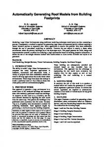
smaller features. As a result less detail of the original model is left out because less points fall into one cluster. Different LODs generated by the method are shown in Fig. 1. Top left shows the original model, the other three groups of pictures show higher LODs of the object in a close-up (big pictures) and magnified versions of both the original model (small left) and the LOD (small right) from a distance for which this LOD is appropriate.

7 A Viewing System Based on Levels of Detail A viewing system using the LODs was implemented both to visually control the results of the method and to demonstrate the usability of the LODs in rendering of complex virtual environments. Generally speaking the incorporation of LODs into the viewer resulted in sufficient speedup for near interactive frame rates (5-10 Hz) on a graphics system with a peak performance of 25K polygons per second. Prior to drawing the scene the system determines the visible objects by classifying their bounding boxes to the viewing frustum. For the potentially visible objects the length of the projection of the bounding box diagonal is calculated to give a measure at which LOD the object should be rendered. Then all the polygons facing the viewer are rendered using the Z-buffer algorithm.

Fig. 2 Living Room left with, right without LODs (left 6810, right 13847 polygons)

8 Results and Timings The proposed method for the automatic generation of LODs works well for polygonal object models of some 1000 vertices. Models can contain any kind of polygons (convex, concave, general) as long as the triangulation algorithm for approximated polygons can handle them. However, convex polygons are preferable for high rendering speed. Lines and points are legal primitives as well. The objects’ meshes should be closed although a violation of this requirement does not prevent the algorithm from being used on the model.

6

Level 0

Original Model

Level 1

Level n

Level 2

Level 3

Fig. 1 Levels of Detail of Plant (6064, 3674, 1225, 339 polygons/lines)

It is possible to vary the method in several ways to better match the requirements of the application 7

for which the LODs are generated. First the number of LODs generated for each object can be adapted by changing the factor by which the dissimilarity measure is updated from level to level. Second the selection of the representative for each cluster can be chosen from a variety of possibilities (cluster average, point in cluster closest to cluster average, point in cluster furthest from object centre, random point in cluster...). Third the primitives generated by the method can be made to include points, lines or polygons or any combination. Fourth the degenerated polygons can be left within the LODs to keep the relationship between the primitives in the original model and the LODs. This is useful for transferring information from the primitives of one LOD to the other (e.g. color, texture, ...). The method was applied to a wide variety of objects achieving acceptable results as far as speed and quality of the approximation are concerned. The resulting LODs are not easily distinguished from the original models when viewed from increasing distances but contain far less polygons than the original models. Fig. 3 shows some more examples of objects and their LODs from a close as well as from a suitable viewpoint, i.e. an appropriate distance for the use of the respective LOD. The statistics of the algorithm are summarized in Table 1 for the objects in Fig. 1 and Fig. 3. They were obtained on a Mips R3000 CPU. Model

Level 0 Polys/Points

Level 1 (polygons)

Level 2 (polygons)

Level 3 (polygons)

Level 4 (polygons)

Time (sec) Total for 4 LOD

Lamp

790 /3084

492 (62%)

210 (27%)

63(8%)

37 (5%)

2.9

Fitting

1581 /5301

1325 (43%)

833 (27%)

225(7%)

55 (2%)

4.2

Shelves

1783 /6628

740 (42%)

472 (26%)

454(25%)

231 (13%)

3.0

Plant

6064 /25926

3674 (61%)

1225 (20%)

339(6%)

57 (1%)

57.0

Table 1 Statistics for the new method

9 Future Work As already mentioned briefly we are investigating at two areas of further research. First we want to further speed up the hierarchical clustering algorithm by making best use of the optimizations described by Murtagh [Murt83]. This work will decrease the order of complexity of the clustering algorithm below O(n2) allowing to deal with more complex object models in less time. Second we want to build a new mode into our viewer which guarantees a constant frame rate through the method described by Funkhouser et al. [Funk93]. We hope to outdo their results in variations in the frame rate as our object models are well structured and probably allow faster and better estimation of the rendering complexity of the visible objects. Further research is needed to increase the flexibility of our method and to further improve the overall look of the LODs. Moreover, we are investigating the applicability of LODs to other application areas.

8

Level 0

Level 0

Lamp Original Model

Level 1

Fitting Original Model

Shelves Original Model Fig. 3 Level of detail close and distant

9

Level 0

Level 0

Level 1

Level 2

Level 0

Level 2

Level 3

Level 0

Level 3

Level 0

Level 1

Level 2

Level 0

Level 3

Level 0

References [DeHa91] Simplification of Objects Rendered - Polygonal Approximations. Michael J. DeHaemer, Jr. and Michael J. Zyda. Computers & Graphics Vol. 15, No.2 pp 175 - 184, 1991. [Funk93] Adaptive Display Algorithm for Interactive Frame Rates During Visualization of Complex Virtual Environments. Thomas A. Funkhouser, Carlo H. Séquin. SIGGRAPH 93, Computer Graphics Proceedings, pp 247-254, 1993. [Hopp94] Piecewise Smooth Surface Reconstruction. Hugues Hoppe, Tony DeRose, Tom Duchamp, Mark Halstead, Hubert Jun, Jon McDonald, Jean Schweitzer, Werner Stuetzle. SIGGRAPH 94, Computer Graphics Proceedings, pp 295-302, 1994. [Murt83] A Survey of Recent Advances in Hierarchical Clustering Algorithms. F. Murtagh.The Computer Journal, Vol. 26, No. 4, 1983. [Rolf94] IRIS Performer: A High Performance Multiprocessing Toolkit for Real-Time 3D Graphics. John Rohlf, James Helman. SIGGRAPH 94, Computer Graphics Proceedings, pp 381-394, 1994. [Ross92] Multi-Resolution 3D Approximations for Rendering Complex Scenes. J. R. Rossignac, P. Borrel. Computer Science, IBM T.J. Watson Research Center, Yorktown Heights, NY 10598, 2 1992. [Rush93] Geometric Simplification for Indirect Illumination Calculations. Holly Rushmeier, Charles Patterson, Aravindan Veerasamy. Proceedings of Graphics Interface ‘93, 1993. [Snea73] Numerical Taxonomy; The Principles and Practice of Numerical Classification. Peter H. A. Sneath, Robert R. Sokal. Publisher W. H. Freeman, San Francisco, 1973. [Turk92] Re-Tiling Polygonal Surfaces. Greg Turk. SIGGRAPH 92, Computer Graphics Proceedings, pp 55-64, 1992. [Schr92] Decimation of Triangle Meshes. William J. Schroeder, Jonathan A. Zarge, William E. Lorensen. SIGGRAPH 92, Computer Graphics Proceedings, pp 65-70, 1992.

10