GB) our tool can, in just over an hour on a standard laptop with two hard drives ... Doing so with existing tools requires powerful computers with very ... raster Digital Elevation Models (DEMs), with good I/O efficiency and the use of only a small ...
Generating Raster DEM from Mass Points via TIN Streaming Martin Isenburg1, Yuanxin Liu 2, Jonathan Shewchuk 1 Jack Snoeyink 2, and Tim Thirion2 1 2
Computer Science Division, University of California at Berkeley Computer Science, University of North Carolina at Chapel Hill
Abstract. It is difficult to generate raster Digital Elevation Models (DEMs) from terrain mass point data sets too large to fit into memory, such as those obtained by LIDAR. We describe prototype tools for streaming DEM generation that use memory and disk I/O very efficiently. From 500 million bare-earth LIDAR double precision points (11.2 GB) our tool can, in just over an hour on a standard laptop with two hard drives, produce a 50,394 × 30,500 raster DEM with 20 foot post spacing in 16 bit binary BIL format (3 GB), using less than 100 MB of main memory and less than 300 MB of temporary disk space.
1
Introduction
Paradoxically, advances in computing capability can make processing more difficult because they enable the acquisition of larger and larger data sets. For example, modern airborne laser range scanning technology (LIDAR) makes it possible to sample large terrains with unprecedented speed and accuracy, obtaining gigabytes of mass points that subsequently must be inspected, processed, and analyzed [1]. Doing so with existing tools requires powerful computers with very large memories. To make this data accessible to the wider audience with commodity computing equipment, we need algorithms that can process large data sets without loading them entirely into memory. Programs that process large data sets must avoid thrashing—spending so much time moving data between disk and memory that computation slows to a crawl. Algorithms have been designed that guarantee the optimal number of disk I/O operations for specific problems [2, 3], at the cost of greater programming complexity. Data layouts have been proposed that are I/O-efficient when accessed with sufficient locality [4, 5], at the cost of an expensive initial re-ordering step. Instead, we advocate a streaming paradigm for processing large data sets, wherein the order in which computations are performed is dictated by the data’s order [6, 7]. We accomplish this by injecting “finalization tags” into a data stream. These tags allow computations to complete early, results to be written to the output immediately, and memory to be reused for incoming data. For stream processing of triangle meshes, Isenburg and Lindstrom [8] propose a streaming mesh format that interleaves vertices, triangles, and vertex
Generation of DEMs via TIN Streaming
Isenburg et al.
finalization tags. Each finalization tag indicates that all the triangles referencing a particular vertex have appeared in the stream, and no more will arrive in the future. A simple stream processing application that benefits from streaming mesh input is computing vertex normals: each incoming triangle adds its normal vector to the vectors for its three vertices. The normal vector for a vertex (the average of its adjoining triangles’ normals) can be computed and output as soon as the vertex’s finalization tag is read from the stream. This topological method of finalizing mesh geometry has many applications, but does not provide a way to process a stream consisting solely of points. So that we may develop streaming point-processing algorithms, we propose in a companion paper [9] to enhance a stream of points with spatial finalization tags. A spatial finalization tag indicates that all the points inside a spatial region have appeared in the stream, and no more will arrive in the future. In Section 2 (and the companion paper), we show how equipping point streams with spatial finalization enables us to compute Delaunay triangulations of huge point sets in a streaming manner. Knowledge about finalized space makes it possible to certify final triangles early, output them, and reuse the memory they were occupying. In this paper, we use both finalized point streams and streaming meshes to link several streaming software modules, which collectively read huge, LIDARgenerated sets of mass points, produce giant TINs, and generate high-resolution raster Digital Elevation Models (DEMs), with good I/O efficiency and the use of only a small memory footprint. Our processing pipeline is illustrated in Figure 1. It consists of three concurrently running processes linked by pipes. A finalizer module, called spfinalize, reads a file of raw mass points and injects spatial finalization tags, producing a finalized point stream. Without touching the disk, this stream is piped into our streaming Delaunay triangulator spdelaunay2d, which writes a TIN in streaming mesh format. As the triangles stream out of the triangulator they are—again without touching the disk—piped into a rasterization module called tin2dem, which uses the triangles and a user-selected interpolation method to estimate elevation values at the raster points of a user-specified elevation grid. Each raster point, with its elevation value, is immediately written into one of many temporary files that are kept open simultaneously; each temporary file stores the raster points for a few rows of the raster DEM. Finally, tin2dem loads these temporary files one by one, sorts the raster points that each one contains into the correct row-by-row ordering, and assembles them into a single, output DEM. The streaming triangulator begins to output TIN data long before it has read all the mass points. Thus it continually frees memory for immediate reuse, so the memory footprint of the triangulator remains small, permitting us to create seamless TINs far larger than the computer’s main memory. The rasterizer writes out raster points as early as possible and, like the triangulator, discards triangles and mass points that are no longer needed. For linear interpolation, it rasterizes and discards each triangle immediately upon reading it. For quintic interpolation, it rasterizes and discards each triangle as soon as all the triangles within a surrounding two-ring have arrived in the input stream (enabling 2 of 13
appeared in GIScience’06
Generation of DEMs via TIN Streaming
Isenburg et al.
Fig. 1. Our pipeline for generating a raster DEM from mass points. A streaming finalizer performs three read passes over the file of raw mass points, and produces a spatially finalized point stream. A streaming Delaunay triangulator reads the finalized mass points from a pipe and produces a streaming TIN mesh, as described in Section 2. A streaming rasterizer reads the streaming TIN, interpolates raster points and stores them to temporary disk files. Then it reads them back one at a time, sorts the points, and produces a single raster DEM, as described in Section 3.
the computation of second-order derivatives at the triangle’s vertices, which are needed for interpolation). When the finalizer, triangulator, and rasterizer run simultaneously, they together occupy a memory footprint that is a small fraction of the sizes of the input and output streams. The order in which the raster points are created depends on the order in which the triangles can be interpolated, which depends on the order of the triangles’ appearance in the streaming TIN, which depends on the order in which regions of space are finalized, which finally depends on the original order of the mass points. For I/O efficiency, the rasterizer does not output raster elevation values directly 3 of 13
appeared in GIScience’06
Generation of DEMs via TIN Streaming
Isenburg et al.
into the final, row-ordered DEM file; instead it writes raster points (i.e. row and column) together with their corresponding elevation values into temporary files on disk. Each file receives several rows’ worth of rasters. After all the triangles are processed, the raster points in the temporary files are read into memory one file at a time. The points in each file are sorted into the correct row and column order, and the elevation values are written to the final DEM in binary BIL format. A special “no data” value is written for those parts of the DEM that did not receive any raster points. As only a few rows of raster points are in memory at any given time, the raster DEM we create can be far larger than the computer’s main memory. This technique can also be used for streaming creation of a DEM from an existing TIN, but requires converting the TIN to a streaming format [8].
2
Streaming Generation of TINs from Mass Points
In the introduction of the DEM Users Manual [1], David Maune says that raster DEMs can be obtained photogrammetrically, however, with most DEM technologies it is more common to first acquire a series of irregularly spaced elevation points from which uniformly spaced elevation points are interpolated. For example, to achieve a uniformly spaced DEM, data producers typically start with mass points and breaklines, produce a TIN, and then interpolate the TIN triangles to obtain elevations at the DEM’s precalculated x/y coordinates. . . . mass points could have been carefully compiled by a photogrammetrist to reflect key spot heights, for example. Alternatively one can imagine hundreds or thousands of similar mass points randomly acquired by a LIDAR or IFSAR sensor. Our goal is to process hundreds of millions of mass points, which can be easily gathered by LIDAR and IFSAR sensors. The technology that enables us to do this is a new, streaming approach for computing Delaunay triangulations [9] that makes it possible to produce billion-triangle TINs on an ordinary laptop computer. A streaming computation reads data sequentially from a disk or a pipe and processes it in memory, confining its operations to the active elements of the stream maintained in a small memory buffer. To keep the size of this buffer small, a streaming computation must be able to finalize elements (e.g., triangles and points) that are no longer needed so they can be written to the output and freed. Unlike with most external memory algorithms, no information is temporarily written to disk; only the output is written. (Our tin2dem module makes a necessary exception to this rule; see Section 3.) Our streaming Delaunay triangulation algorithm [9] is based on the idea of enhancing a point stream with spatial finalization. Finalization is a technique for improving the efficiency of streaming computation by including in the stream some information about the future of the stream. The triangulator’s input stream is not just a list of points—it also contains spatial finalization tags that inform 4 of 13
appeared in GIScience’06
Generation of DEMs via TIN Streaming
Isenburg et al.
our Delaunay triangulator about regions of space for which the stream is free of future points. The purpose of these tags is to give our algorithm (or other point processing applications) guarantees that allow it to complete computation in finalized regions, to output triangles (or other data) that can be certified to be part of the correct solution, and to reuse the memory those triangles were occupying—long before all the points in the input stream have been read. We define a spatially finalized point stream to be a sequence of entities, of which all but one are points or finalization tags. The first entity in the stream is special: it specifies a subdivision of space into regions. We use a rectangular 2k × 2k grid of cells as our subdivision. Hence, the stream begins by specifying a bounding box (which encloses all the points in the stream, and defines the grid of cells) and the integer k (which defines the resolution of the grid). The remainder of the stream is points and tags. Immediately after the last point that falls in a given cell of the grid, we insert a finalization tag that certifies that no subsequent point in the stream falls into that cell. Our Delaunay triangulator uses the spatial finalization tags to certify triangles as final. A triangle is final when its circumcircle is completely inside the union of the finalized cells. When a triangle is final, it can be written to the output and its memory can be freed to make room for more data to stream in. Before a triangle is written we check whether its three vertices have already been referenced before and if not, first write them to the output. Once all triangles adjoining a vertex are final, the vertex can likewise have its memory freed. The output is written in a streaming mesh format [8], described briefly in Section 1. We have implemented streaming two- and three-dimensional Delaunay triangulators by taking existing sequential Delaunay triangulators, based on the well-known incremental insertion algorithm [10–12], and modifying them so that they retain in memory only the active (non-final) parts of the triangulations they are constructing. (We will discuss only the two-dimensional triangulator in this paper.) Because the triangulator constantly outputs and deallocates triangles and vertices, its memory footprint remains small throughout execution. This makes it possible to compute seamless TINs for huge point sets. Where do we get a finalized point stream? Ideally, we advocate that programs that create huge point sets should include finalization tags in their outputs. We believe that this option will become increasingly attractive as huge data sets become more common, because it is usually easy to implement, and if it is not implemented, users will not be able to process those data sets on commodity computers without I/O heavy operation to prepare the data. However, we also have written software called a finalizer that adds finalization tags to a point stream as a preprocessing step. An important feature of our finalizer is that its output can be piped directly to another application, notably our triangulator, so there is no need to store the finalized point stream on disk. Our finalizer makes three read passes over a raw point file, and writes a finalized point stream to the output during the third pass. During the first pass, it computes a rectangular, axis-aligned bounding box of the points. The finalization regions are defined by the subdivision of this bounding box into a 5 of 13
appeared in GIScience’06
Generation of DEMs via TIN Streaming
Isenburg et al.
2k × 2k grid of uniform cells. The second pass counts how many input points lie in each cell. The third pass uses these counts to find the last point in each cell, and to insert a finalization tag immediately after it. The finalizer also reorders the points, so that all the points that lie in one cell appear contiguously in the stream. Specifically, for each cell of the grid, the finalizer stores the points that lie in the cell in a memory buffer until all the cell’s points have arrived. Then it outputs all the cell’s points at once into the finalized point stream, followed by a finalization tag for the cell. One motivation for delaying points in the stream is the fact that each point inserted into a triangulation adds far more memory (for triangulation data structures) to the triangulator’s memory footprint than the point would occupy in the finalizer’s memory buffers. Therefore, it is beneficial to put off inserting a point until it has a chance to become final in the near future. Another motivation is to improve the speed of point location in the incremental Delaunay insertion algorithm, by keeping the number of triangles small. We triangulate huge raw point sets by running our finalizer software, spfinalize, and our Delaunay triangulator, spdelaunay2d, concurrently while piping the finalizer’s output, a finalized point stream, directly into the triangulator (see Figure 1). The two processes together triangulate the 11.2 GB of bare-earth LIDAR data for the Neuse River Basin of North Carolina, which consists of over 500 million points (double-precision x, y, and elevation coordinates), in 48 minutes on an ordinary laptop computer, while using 70 MB of memory. This time includes the finalizer’s three read passes over the raw input points stored on disk, and the triangulator’s concurrent writing of a streaming mesh to disk. It is about a factor of twelve faster than the previous best out-of-core Delaunay triangulator, by Agarwal, Arge, and Yi [3]. With our streaming Delaunay software, we have constructed triangulations as large as nine billion triangles, in under seven hours using as little as 166 MB of main memory [9].
3
Mass Points to DEM
In this section, we discuss our software pipeline for converting mass points into a DEM. We assume that the user has specified the output raster grid, usually by giving the northing, easting, and grid resolution. Our task is first to create a seamless TIN, then to interpolate elevation values at the grid points and create a single raster DEM for output. The first part of our pipeline is the streaming Delaunay triangulator described in the previous section, which creates the TIN. The second part is software that uses the TIN triangles to interpolate the elevation at the raster points defined by the raster grid, then collects the resulting raster points into a single global DEM in some standard order. We consider rasterizing and ordering in the following two subsections. 3.1
Rasterizing the Streaming TIN
We make the following choices for our implementation. 6 of 13
appeared in GIScience’06
Generation of DEMs via TIN Streaming
Isenburg et al.
– We take in points with UTM coordinates in a single zone. It is a simple matter of programming to customize the software to user requirements such as generalizing to multiple zones or geographic (latitude/longitude) coordinate systems. The selected interpolation function needs to match the coordinate system, of course. – We reject triangles that have an edge longer than a user-defined threshold from being rasterized. This prevents interpolating the elevation across large triangles that can only exist in areas without LIDAR data. These areas are not LIDAR mapped but are inside the convex hull of the LIDAR points, including water surfaces where LIDAR does not give any returns. – We use linear or quintic interpolants based on TIN triangles. Other forms of interpolation could also be supported, but these two are popular, and they demonstrate key concepts. The linear interpolant requires information from only a single triangle. It is primarily I/O-bound, so it shows the best improvement from streaming. The quintic interpolant [13] requires neighbor information to estimate first and second derivatives at each vertex. This requires more computation and more buffering, as we need two rings of surrounding triangles to compute estimates for the second derivative. – We output the results to a single DEM in a binary format, primarily to show that our computation is seamless. Of course, a 12 gigabyte raster DEM stored as a single file in row-ordered BIL format is not useful for most applications that use DEM files, because they do not (yet) use streaming computation. We could instead produce tiled output that can be ingested by GIS systems, but we decided to make a single DEM as a proof of concept and I/O-efficiency. Writing tiles or other orderings as output is an easy modification. 3.2
Row-Ordering of Streaming Raster Points
The rasterizer produces the elevation values that make up a raster DEM, but does not produce them in the order that they need to appear in the file—instead, raster points are written out in the order triangles are interpolated, so that the triangles’ memory can be freed up to make room for more incoming TIN data. Since we know the file location where each raster point will ultimately go, we could write it there using random access to a file (or equivalently, using memory mapping and relying on the operating system to swap portions of the elevation data between memory and disk). This strategy is slow because the file is stored in a row-order layout and the interpolator accesses the rows in a random-access manner, entailing many distant disk seeks. Thrashing can be reduced (but not eliminated) by buffering several raster points per row before writing them to disk. The approach has other disadvantages too: it entails an initial pass over the entire file to initialize the entire DEM with “no data” raster points, and a final pass if the DEM is to be stored in a compressed format. Moreover, some computer systems limit main memory address space mapping and random file access (e.g. fseek) to under 2 GB, which is not quite enough to store a 32,678 × 32,768 grid with 16-bit elevation values. We want to create larger DEMs. 7 of 13
appeared in GIScience’06
Generation of DEMs via TIN Streaming
Isenburg et al.
Agarwal et al. [14] use an alternative approach. They write each interpolated elevation raster point with its column and row address to a temporary file. After all the raster points are written, they use an external sorting algorithm to bring the raster points into their proper order. This strategy produces a temporary file that is two or three times the size of the final DEM, as the column/row address of a raster point often requires more bytes of storage than the actual elevation value. Because this temporary file is used as input to a generic external sorting algorithm it is not possible to store its contents in compressed form. We found that a hybrid approach gives the best overall performance. We maintain many temporary files, each representing a few consecutive rows of the output DEM. In memory, we maintain for each temporary file a small buffer of raster points and write out a buffer whenever it fills up. To save temporary disk space, we devised a fast compression scheme that avoids redundant bits when writing a full buffer to disk: raster points are grouped by row; within each row, the raster points are sorted by column and runs of columns are combined (so that a column number does not need to be stored for every point); and elevation values are encoded as differences. The contents of one temporary file are small enough to fit uncompressed in main memory. After the rasterizer finishes processing the streaming TIN data, it decompresses the temporary files one at a time, sorts the raster points into the correct row and column ordering, and outputs them into the final DEM file while putting “no data” values wherever there are no raster points. Our use of multiple temporary files can be seen as a preliminary bucket sort step, which makes the subsequent sorting steps fit in memory.
4
Experimental Results
In Table 1 we report performance, in terms of computation time, main memory use, and temporary disk space, for our streaming pipeline as it generates raster DEMs of various resolutions from LIDAR-collected mass points. The measurements are taken on a Dell Inspiron 6000D laptop with a 2.13 GHz mobile Pentium processor and 1 GB of memory, running Windows XP. The point file is read from, and the DEM file is written to, an external LaCie 5,400 RPM firewire drive, whereas the temporary files are created on the 5,400 RPM local hard disk. Each run takes as input a binary 11.2 GB file that contains 500,141,313 points in double precision floating-point format, and produces as output a raster DEM in binary BIL format with 16-bit elevations. As points are read from disk they are converted to single-precision floating-point format, which provides sufficient precision for our purpose. Each run constitutes a pipeline of three stream modules (see the command line in the table) that operate in four steps. The first two steps could be omitted if the input points were stored in a format that provides spatial finalization. 1st step. A read pass over the points by spfinalize allows it to compute the bounding box. This pass is strictly I/O-limited as it takes 6 minutes to read 11.2 GB from disk. 8 of 13
appeared in GIScience’06
Generation of DEMs via TIN Streaming number of points, file size LIDAR [minx ; maxx] input mass points [min y; maxy] [minz ; maxz ]
Isenburg et al. 500,141,313 11.2 GB [1,930,000; 2,937,860] [ 390,000; 1,000,000] [ −129.792; +886.443]
spfinalize -i neuse.raw | spdelaunay2d -ispb -osmb | tin2dem -ismb -o neuse.bil -xydim 20
grid spacing 40 ft cols 25,198 rows 15,250 output file size 750 MB Time (hours:minutes) total 0:53 bounding box 1st step 0:06 finalization counters 2nd step 0:06 finalize, triangulate, raster, scratch 3rd step 0:40 read scratch, sort, write final 4th step 0:01 Memory (MB) maximum 55 spfinalize (1st step) .1 spfinalize (2nd step) 5 spfinalize (3rd step) 35 spdelaunay2d (3rd step) 10 tin2dem (3rd step) 10 tin2dem (4th step) 38 Scratch Files (MB) total size 82 (compressed) number of files 60 rows per file 256 number of written raster points in millions 111 storage & I/O savings—raw : compressed 8.0 : 1 DEM output grid
20 ft 10 ft 50,394 100,788 30,500 61,000 3.0 GB 12.0 GB 1:07 1:20 0:06 0:06 0:06 0:06 0:43 0:48 0:08 0:20 64 91 .1 .1 5 5 35 35 10 10 19 35 46 91 270 868 239 477 128 128 444 1,767 9.6 : 1 11.9 : 1
Table 1. Statistics for an input data set of 500 million LIDAR-collected mass points of the Neuse River Basin, from which we compute DEM grids with 40, 20, and 10 foot spacing using linear interpolation. We give an example of how three processes are piped together on the command line. We report time, memory use, and disk use for each step of the computation and each module in the pipeline, at each resolution.
2nd step. Another read pass over the points by spfinalize is used to count the mass points lying in each cell of a 29 × 29 grid derived from the bounding box. These counts are used in the next step for spatial finalization. This pass is also I/O-limited, and again takes 6 minutes. So far, relatively little main memory is used. 3rd step. During the third read pass over the points, a pipeline of three processes do the real work: spfinalize adds finalization tags to the stream of points and pipes space-finalized points to spdelaunay2d, which immediately begins to triangulate the points and pipes a streaming TIN onward to tin2dem, which begins to rasterize incoming triangles onto the DEM grid as early as possible, and writes raster points grouped by rows into temporary files on the second hard drive. This step is CPU-limited, with the three processes sharing the available CPU cycles. The proportion of the workload 9 of 13
appeared in GIScience’06
Generation of DEMs via TIN Streaming
Isenburg et al.
carried by tin2dem increases as the DEM grid resolution becomes finer, as more interpolation operations are performed per triangle. The memory footprint is that of all three processes combined: spfinalize requires 35 MB, most of which goes toward delaying the points in a cell until all the cell’s points arrive. spdelaunay2d requires 10 MB for streaming Delaunay triangulation. The memory requirements of tin2dem depend only on how many raster points are accumulated per DEM row before they are written to a temporary file in compressed form. For the results we report in the table, each DEM row has its own memory buffer, whose contents are compressed and written to disk when 64 raster points accumulate. Each raster point occupies six bytes—two for the elevation and four for the column index—so the 10-foot resolution DEM with 61,000 rows occupies a 35 MB memory footprint. All three processes together occupy 104 MB. 4th step. In this step, only the tin2dem process is still running. It loads the temporary files into memory, one at a time; sorts the rasters into the correct row and column order; and outputs them to a binary file in BIL format, while filling in missing raster points with the number −9999, which represents “no data.” This final step, like the first two, is I/O-limited, and the disk throughput is the bottleneck. We would significantly reduce the amount of data written to disk, and realize faster running times, if we replaced the uncompressed BIL format with a compressed format for DEMs. The memory footprint of tin2dem is larger during the 4th step than during the 3rd, because it must simultaneously store in memory all the raster points from one temporary file. For the 10-foot resolution DEM, each temporary file contains 128 rows of up to 100,788 rasters each, so the memory footprint is 91 MB. (Some potential for memory reuse is left untapped.)
Fig. 2. Two snapshots during streaming construction of a DEM grid from the LIDARcollected mass points of the Neuse River Basin. Blue cells are unfinalized space, violet triangles are non-final Delaunay triangles, color-shaded areas contain elevation rasters that have already been generated, and the grey LIDAR points inside the blue cells have not yet streamed into the triangulator.
Recent work by Agarwal et al. [14] also describes a method for constructing DEM grids from huge LIDAR data sets. They report an end-to-end running 10 of 13
appeared in GIScience’06
Generation of DEMs via TIN Streaming
Isenburg et al.
time of 53 hours for rasterizing the 20 foot DEM of the Neuse River Basin. This is much slower than the one hour and 16 minutes we report, but most of the difference is attributable to their much more complex interpolation method [15], which takes 86% (46 hours) of their computation time. Most of the remaining seven hours are spent finding neighboring mass points that are needed by the interpolator. This is where we believe our data-driven approach can shine: we do not have to spend any time gathering neighbor data for our computations. The arrival of sufficient neighbor data is what determines when a computation is performed. However, we are not yet in a position to make a direct comparison between our DEM creation software and that of Agarwal et al.
5
Discussion
The prototype workflow described in this paper can take huge numbers of mass points, build monstrously large, seamless TINs, and output high-resolution raster DEMs. We achieve this with a streaming, data-driven paradigm of computation and an off-the-shelf laptop, using main memory resources that are just a fraction of the size of the input and the output. Our processing pipeline uses spatial finalization of points to enable streaming Delaunay computation, and vertex finalization in the resulting TINs to enable streaming interpolation of elevations and the production of streams of raster points. Streaming algorithms can succeed only if streams have sufficient spatial coherence—a correlation between the proximity in space of geometric entities and the proximity of their representations in the stream. Fortunately, our experience is that huge real-world data sets usually do have sufficient spatial coherence. This is not surprising; if they didn’t, the programs that created them would have bogged down due to thrashing. (Our finalizer also increases the stream’s spatial coherence by reordering the points.) For data sets with no spatial coherence at all, however, we advocate an external sort of the points before finalizing them. Our tin2dem tool can process pre-existing TIN data. First, however, each TIN needs to be converted to a streaming mesh format, with interleaved vertices, triangles, and vertex finalization tags. For large TINs whose vertices and triangles are ordered with little spatial coherence, this conversion can be expensive [8]. If a TIN is spatially coherent enough, however, a simple streaming conversion method is to make one pass over the TIN file. As soon as a vertex is surrounded by a complete star of triangles, we guess that the vertex can be finalized and inject a finalization tag for it into the stream. Many other GIS processing tasks could be implemented as streaming computations, enabling them to handle huge data sets. Slope and aspect could be produced immediately by the linear or quintic interpolator. Mass points could come from photogrammetry, IFSAR, or contour lines, instead of from LIDAR. To support breaklines, we plan to extend our streaming Delaunay triangulator to construct constrained Delaunay triangulations. For this to remain efficient, we will need streaming input files that encode both points and breaklines in a spa11 of 13
appeared in GIScience’06
Generation of DEMs via TIN Streaming
Isenburg et al.
tially coherent order. We will also need to devise a method of spatial finalization that takes into account both points and breaklines. Other forms of interpolation could be streamed too. Streaming natural neighbor (or area-stealing) interpolation [16–18] is straightforward to implement, as the Delaunay triangulation is already available. Interpolation methods that compute weighted averages of the k nearest neighbors (typically with 6 ≤ k ≤ 12) can also be implemented in a streaming manner, but it takes some care to devise an algorithm that ensures that the streaming interpolator does not hold too many points in memory, yet does not discard a point that might be a near neighbor of some future point in the stream. Interpolation methods that use global radial basis functions are not suitable for streaming, or even for global use on large data sets. They can be made a little more suitable by building them into a quadtree, as is done for the regularized spline with tension (RST) [15] implemented in GRASS. However, Agarwal et al. [14] has an external memory implementation of a restricted variant of the RST, which uses a bitmap to enforce the locality of the computation, and they compare it to the RST implementation in GRASS. RSTs are not intended to provide a fast, turnkey interpolant, so it is no surprise that they do not work effectively with massive data sets. Their real advantage is having many parameters to tune, to help fit specific characteristics to portions of the landscape. It will be more challenging to apply streaming to less local operations, such as hydrological enforcement [19]. Hydrological enforcement adjusts elevations to respect water flow, so that bridges and culverts do not look and behave like dams. We think that these adjustments could be performed in a streaming manner if summary information on water flow were collected and buffered. We would like to hear from people who have a specific application and data sets that could benefit from streaming. Suitable applications are those whose operations have some spatial locality, although the degree of locality might be determined by the data. Obvious candidates for streaming are filtering operations that prepare the raw LIDAR data for subsequent processing, such as extraction of bare-earth returns and point thinning for excessively dense data. Acknowledgments. We thank Kevin Yi for supplying the Neuse Basin data and Andrew Danner for extensive information about his work [14]. This work was supported by National Science Foundation Awards CCF-0430065 and CCF-0429901: “Collaborative Research: Fundamentals and Algorithms for Streaming Meshes,” National Geospatial-Intelligence Agency / Defense Advanced Research Projects Agency Award HM1582-05-2-0003, and an Alfred P. Sloan Research Fellowship.
References 1. Maune, D.F., ed.: Digital elevation model technologies and applications: The DEM users manual. ASPRS, Bethesda, MD (2001) 2. Vitter, J.S.: External memory algorithms and data structures: Dealing with MASSIVE data. ACM Computing Surveys 33(2) (2001) 209–271
12 of 13
appeared in GIScience’06
Generation of DEMs via TIN Streaming
Isenburg et al.
3. Agarwal, P.K., Arge, L., Yi, K.: I/O-efficient construction of constrained Delaunay triangulations. In: Proceedings of the Thirteenth European Symposium on Algorithms. Volume 3669 of LNCS., Mallorca, Spain, Springer Verlag (2005) 355–366 4. Cignoni, P., Montani, C., Rocchini, C., Scopigno, R.: External memory management and simplification of huge meshes. IEEE Transactions on Visualization and Computer Graphics 9(4) (2003) 525–537 5. Yoon, S., Lindstrom, P., Pascucci, V., Manocha, D.: Cache-oblivious mesh layouts. ACM Transactions on Graphics 24(3) (2005) 886–893 6. Isenburg, M., Gumhold, S.: Out-of-core compression for gigantic polygon meshes. ACM Transactions on Graphics 22(3) (2003) 935–942 7. Isenburg, M., Lindstrom, P., Gumhold, S., Snoeyink, J.: Large mesh simplification using processing sequences. In: Visualization ’03 Proceedings. (2003) 465–472 8. Isenburg, M., Lindstrom, P.: Streaming meshes. In: Visualization ’05 Proceedings. (2005) 231–238 9. Isenburg, M., Liu, Y., Shewchuk, J., Snoeyink, J.: Streaming computation of Delaunay triangulations. ACM Transactions on Graphics 25(3) (2006) Special issue on Proceedings of ACM SIGGRAPH 2006. 10. Lawson, C.L.: Software for C 1 Surface Interpolation. In Rice, J.R., ed.: Mathematical Software III. Academic Press, New York (1977) 161–194 11. Bowyer, A.: Computing Dirichlet Tessellations. Computer Journal 24(2) (1981) 162–166 12. Watson, D.F.: Computing the n-dimensional Delaunay Tessellation with Application to Voronoi Polytopes. Computer Journal 24(2) (1981) 167–172 13. Akima, H.: A method of bivariate interpolation and smooth surface fitting for irregularly distributed data points. ACM Transactions on Mathematical Software 4 (1978) 148–159 14. Agarwal, P.K., Arge, L., Danner, A.: From LIDAR to grid DEM: A scalable approach. In: Proc. International Symposium on Spatial Data Handling. (2006) 15. Mitasova, H., Mitas, L.: Interpolation by regularized spline with tension: I. Theory and implementation. Mathematical Geology 25 (1993) 641–655 16. Gold, C.M.: Surface interpolation, spatial adjacency and GIS. In Raper, J., ed.: Three Dimensional Applications in Geographic Information Systems. Taylor and Francis, London (1989) 21–35 17. Sibson, R.: A brief description of natural neighbour interpolation. In Barnett, V., ed.: Interpreting Multivariate Data. John Wiley & Sons, Chichester (1981) 21–36 18. Watson, D.F.: Natural neighbour sorting. Australian Computer Journal 17(4) (1985) 189–193 19. Hutchinson, M.F.: Calculation of hydrologically sound digital elevation models. In: Proceedings of the Third International Symposium on Spatial Data Handling. (1988) 117–133
13 of 13
appeared in GIScience’06