Generating Realistic Heterogeneous Agents: Computing Confidant-based Base Interaction Probabilities Alex Yahja Carnegie Mellon University
[email protected] Kathleen M. Carley SDS, Carnegie Mellon University
[email protected] Abstract Organizational theory often assumes classes of agents, for example classes of the operating core, the middle line, the strategic apex, the techno-structure, and support staff. While these classes are adequate for conventional analysis of organization, they are inadequate for more sophisticated analysis using computer modeling and simulation. Furthermore, in reality, organizational agents – humans, software agents, webbots or robots – are very complex and exhibit a plethora of behaviors. Modeling such agents with sufficient accuracy is a challenge. We take a statistical approach to model the behavior of these agents in this paper. We are modeling the interaction probabilities between two categories of agents so that the number of confidants (the number of people each agent interacts with most) matches the empirical population data about confidants. A gradient descent approach is used and the results are presented indicating the efficacy of the approach. This work represents the first step in generating heterogeneous organizational agents based on empirical data and its use in enhancing the evaluation of organization theory by computer-enabled theorizing. Contact: Alex Yahja Engineering and Public Policy Department Carnegie Mellon University Pittsburgh, PA 15213 Tel: 1-412-374-9375 Email:
[email protected] Key Words: heterogeneous organizational agents, gradient descent, confidants, computational organization theory Acknowledgement: This work was supported by contract 290-00-0009 from the Defense Advanced Research Projects Agency, by the Agency for Healthcare Research and Quality; Cooperative Agreement Number U90/CCU318753-01 and UP0/CCU318753-02 from the Centers for Disease Control and Prevention (CDC), by the NSF IGERT in CASOS, and the Carnegie Mellon center for Computational Analysis of Social and Organizational Systems. Its contents are solely the responsibility of the authors and do not represent the official views of DARPA, the CDC, or the NSF.
Generating Realistic Heterogeneous Agents: Computing Confidant-based Base Interaction Probabilities Organizational theory often assumes classes of agents, for example classes of the operating core, the middle line, the strategic apex, the techno-structure, and support staff [Mintzberg, 1979]. While these classes are adequate for conventional analysis of organization [Evan, 1993], they are inadequate for more sophisticated analysis using computer modeling and simulation. Furthermore, in reality organizational agents – humans, software agents, or robots -- are very complex and have complex behaviors, so attempts to model them in sufficient accuracy is a challenge [Carley and Newell, 1994]. We take the statistical approach to model the behavior of these agents in this paper. We are modeling the interaction probabilities between two categories of agents so that the number of confidants (the number of people each agent interacts with most) matches the empirical population data about confidants. Gradient descent approach is used and the results are presented indicating the efficacy of the approach. This work represents the first step in generating heterogeneous organizational agents based on empirical data and its use in enhancing the evaluation of organization theory by computer-enabled theorizing. Motivation for this study was based on preliminary results of the Biosurveillance project. In the project, a social interaction model CONSTRUCT [Carley, 1990] and a disease model are combined to predict the propagation of a bioattack and evaluate possible response policies. In the effort to model the reality better, we have a need to generate heterogeneous agents, which as a population match the empirical population data. In this paper we assume an asymmetric interaction model. Prietula gave examples of asymmetric interaction model in the trust and advice networks [Prietula, 2000]. The problem of generating heterogeneous agents is one of organization’s problems because most if not all organizations contain heterogeneous agents. If we are to model organization in a greater precision and fidelity, we need to have realistic heterogeneous agents. “Realistic” here means realism in term of sociological, geographical, institutional, organizational, demographical, symbolic-mythical, cognitive, network, biological, and psychological factors. The paper by Huchins supports this proposition of the need for realistic heterogeneous agents, as (individual) cognition does not take place outside or divorced from culture, history, emotion, climate, etc [Huchins, 1995]. In this paper, we will use the term of “heterogeneous agents” to convey the notion of heterogeneous agents that are realistic on multiple fronts.
Previous Work on Heterogeneous Agents There is little work done so far in (realistic) heterogeneous agents [Prietula et. al., 1998][Carley and Prietula, 1994]. So we will describe work related to heterogeneous agents and to where heterogeneous agents could have an impact. The closest work to creating heterogeneous agents is the work of Plural-Soar, which is heterogeneous and logically and organizationally somewhat realistic [Carley et al, 1992]. However this Plural-Soar is not a full social agent. A major aspect of creating a social agent is the specification of social and cultural knowledge for the agent. Realistic agents across broader spectrum of fields demand even more specifications, which could include geographical, institutional, network, symbolic-mythical, and other knowledge and behaviors. Most work on organization theory assumes homogeneous agents. Early work on organization theory assumes black box abstraction of classes of agents. Mintzberg described five basic parts of the organization [Mintzberg, 1979], abstracting classes of agents by organizational chart. The Garbage Can model [Carley, 1986] also abstract agents into aggregate black boxes. Most work on multi-agent systems does not consider socially, demographically, geographically, culturally, cognitively realistic network agents. In the field of computational organizational theory [Carley and Gasser, 1999], the need for heterogeneous agents is implied by the nature of organizations, which is heterogeneous. The computational approach to theorizing about organization is necessary because organizations are heterogeneous, complex, nonlinear dynamic adaptive and evolving systems. Organizations have emergent structuration and hundreds of interaction, thus making it poor candidates for analytical models. Organizations are social systems [Parsons, 1990], thus the naturally occurred socially heterogeneous agents affect organizations. There is work on modeling organizational adaptation as a simulated annealing process, and by genetic algorithms, but they assume the unit of analysis – the agent – is homogeneous. Friedland and Alford in their paper [Friedland and Alford, 1991] pointed out the need of realistic social science, which does not blindly adhere to a materialist-idealism false dualism, but considers individual behavior,
organizational action, and institutional relationships. This individual behavior is complex and as individuals are naturally heterogeneous, the need for heterogeneous agents is self-evident. Masuch and LaPotin proposed DoubleAISS model as an improvement to Garbage Can model [Masuch and LaPotin, 1989]. DoubleAISS includes an actor model, which takes into account issues, skills, structure & authority relations, and actions, which are a subset of organizational factors. This agent model however is not heterogeneous. Levinthal described modeling adaptation on rugged landscape for organizations [Levinthal, 2001]. The unit of analysis here is organization not individual agent. The notion of adapting organizations via dynamic of search on rugged environments could extend to the notion of adapting agents on their organizational and sociological environments. As agents are naturally heterogeneous, the question of how to adapt agents to their organizations necessitates the research of building heterogeneous agents. Heterogeneous agents, as they would include culture in the final form, are essential to understanding the culture of organization and social systems. Ouchi and Wilkins provided a comprehensive survey of organizational culture research [Ouchi and Wilkins, 1985]. Complex multi-cultural agents give rise to complex multi-cultural organizations. Louis proposed organizations as culture-bearing milieux, that is, as distinctive social units possessed of a set of common understandings for organizing action and languages and other symbolic vehicles for expressing common understanding [Louis, 1980]. Thus in order to research organizational culture precisely, we need to have heterogeneous agents capable of bearing culture. Another paper by Schein provided the definition of organizational culture [Schein, 1996]. Values and philosophy arose from interaction between heterogeneous agents and between these agents and their physical environments. Thus heterogeneous agents are necessary to understanding organizational culture. On a higher level, cultures are transmitted among organizations in many different ways via hiring, socialization, and turnover [Harrison and Carroll, 1991]. Furthermore the need of heterogeneous agents is related to high reliability organizations, because in recognizing the nature of organizational agents, which are heterogeneous, we could better analyze whether an organization meets the criteria for high reliability. Roberts described the findings on a project concerned with the design and management of hazardous organizations that achieve extremely high level of reliable and safe operations [Roberts, 1989].
Empirical Data We use two sets of empirical categorical data. This data is a population-level data, describing the number of confidants (the number of people you interact most) for each class of agents. The data is the national average for the number of confidants. The data is suitable for this research, as it provides the empirical grounding essential for building realistic heterogeneous agents. Table 1 shows the mean and standard deviation of confidants and the number of agents in each class of the AGE categorical data.
Table 1: The mean and standard deviation of confidants for AGE category
Report NUMGIVEN AGE Mean 5 15.00 3.5789 20.00 3.2391 25.00 3.4041 30.00 3.4167 35.00 3.1988 40.00 3.0750 45.00 3.1400 50.00 2.9545 55.00 2.8070 60.00 2.8879 65.00 2.3434 70.00 2.1096 75.00 2.0370 80.00 1.5385 85.00 1.9500 Total 2.9692
N 19 138 193 180 161 120 100 110 114 107 99 73 54 39 20 1527
Std. Deviation 1.2612 1.4825 1.6210 1.5459 1.6576 1.6861 1.9176 1.7047 1.7442 2.1471 1.7564 2.0921 1.6706 2.3152 1.6376 1.7955
The first entry of the table shows that the class of age 15 to 19 has 19 agents total, and has the mean of 3.5789 confidants with a standard deviation of 1.2612. Note that the mean number of confidants is not integer, because it is averaged over the number of agents. “AGE 5” in the table above means the interval of 5 years. We redisplay the above table to graph for clarity. Thus graphically, Figure 1 below depicts the mean.
4.0
3.5
Mean NUMGIVEN
3.0
2.5
2.0
1.5 15.00
25.00
20.00
35.00
30.00
45.00
40.00
55.00
50.00
65.00
60.00
75.00
70.00
85.00
80.00
AGE5
Figure 1: Graph of Mean for AGE Category Figure 2 shows the standard deviation for AGE categorical data. 4.0
3.5
95% CI NUMGIVEN
3.0
2.5
2.0
1.5 N=
19
138
15.00
192
180
25.00
20.00
161
120
35.00
30.00
100
110
45.00
40.00
113
105
55.00
50.00
98
72
65.00
60.00
54
37
75.00
70.00
20
85.00
80.00
AGE5
Figure 2: Graph of Standard Deviation for AGE Category
Table 2 below shows the mean and standard deviation of confidants and the number of agents for EDUCATION categorical data.
Table 2: The mean and standard deviation of confidants for EDUCATION category Report NUMGIVEN Education .00 1.00 2.00 3.00 4.00 5.00 6.00 7.00 8.00 9.00 10.00 11.00 12.00 13.00 14.00 15.00 16.00 17.00 18.00 19.00 20.00 Total
Mean .3333 2.0000 2.0000 1.7778 2.7500 2.5556 1.7368 1.6667 1.8023 2.4444 2.2093 2.5700 2.8121 3.1626 3.5564 3.6892 3.6809 3.9783 4.0000 3.9167 4.0938 2.9596
N 3 2 6 9 8 9 19 27 86 63 86 100 511 123 133 74 141 46 44 12 32 1534
Std. Deviation .5774 1.4142 2.0000 1.4814 1.4880 2.1858 1.7270 1.4142 1.5705 1.6439 1.5950 1.9708 1.7320 1.8964 1.6579 1.4611 1.6315 1.6260 1.5250 1.5050 1.2536 1.7997
The first entry in the table above shows that there are 3 agents who have 0 to less than 1 years of schooling (the number in the “Education” column means the number of years schooling, 12 = high school graduate, 16 = college graduate, etc.), and who have 0.3333 confidants with a standard deviation of 0.5774. Graphically, Figure 3 shows the mean for EDUCATION categorical data.
5
4
Mean NUMGIVEN
3
2
1
0 .00
2.00
4.00
6.00
8.00
10.00 12.00
14.00 16.00
Education
Figure 3: Graph of Mean for EDUCATION Category
Figure 4 below shows the standard deviation for EDUCATION categorical data.
18.00 20.00
5
4
95% CI NUMGIVEN
3
2
1
0 N= 3
.00
2
6
2.00
9
8
4.00
9
19 27 86 63 86 100 511 123 133 74 141 46 44 12 32
6.00
8.00 10.00 12.00 14.00 16.00 18.00 20.00
Education Figure 4: Graph of Standard Deviation for EDUCATION Category
Gradient Descent Approach As described earlier, we have the task of setting the base interaction probabilities between agents so that the mean and standard deviation of the number of confidants agree with the empirical national average data. Note that in this paper we only attempt to create a very small subset of realism for agents. We use the gradient descend approach to fit the base interaction probabilities so that the resulting number of confidants for all categories meets the national average empirical data. In this work, we assume the matrix of interaction is asymmetric. The algorithm is as follows: Repeat till both errors of mean and standard deviation are smaller than EPSILON, a very small number Randomly choose a cell, and choose an addition of positive or negative DELTA, a small increment, to the cell’s number content (a cell contains the interaction probabilities of a pair of agents) If the new number makes both the absolute errors of mean and standard deviation smaller, Then keep the new number Else we go in another direction (if the previous DELTA is positive, we now take the negative) End-of-if End-of-repeat To determine who is a confidant, we set a threshold, the confidant threshold, to be 0.55. The number of confidants is calculated by #confidants/agent = (INTEGER) (N1 * (N2-1) * max(interaction probability - confidant threshold, 0)) / N1 where N1 is the number of agents in the class agent 1 belongs to, N2 is the number of agents in the class agent 2 belongs to. ”( INTEGER)” means rounding to the nearest integer.
Results We will show the results and at the same time go through the computational steps. First we combine the two categories into a single interaction probabilities matrix. After the gradient descent algorithm is run, this interaction probabilities matrix shows the base interactions probabilities needed for agents to meet the national average of the number of confidants. (And indeed, the interaction probabilities matrix below shows the resulted base probabilities.)
INTERACTION PROBABILITIES:
N1
N2
19
138
193
180
161
120
100
110
11
Category
15
20
25
30
35
40
45
50
5
19
15
0.6
0.6
0.56
0.57
0.57
0.6
0.7
0.6
0
138
20
0.61
0.56
0.56
0.6
0.56
0.61
0.7
0.6
0
193
25
0.59
0.595
0.595
0.59
0.59
0.59
0.59
0.59
0.5
180
30
0.61
0.58
0.58
0.58
0.58
0.59
0.59
0.61
0.6
161
35
0.6
0.58
0.58
0.58
0.58
0.59
0.6
0.6
0
120
40
0.6
0.58
0.58
0.58
0.58
0.58
0.58
0.59
0.58
100
45
0.6
0.58
0.58
0.58
0.585
0.58
0.58
0.6
0.5
110
50
0.58
0.58
0.58
0.58
0.58
0.58
0.58
0.58
0.5
114
55
0.6
0.58
0.58
0.58
0.58
0.58
0.6
0.58
0.5
107
60
0.6
0.58
0.58
0.58
0.58
0.58
0.58
0.58
0.5
99
65
0.57
0.58
0.58
0.58
0.58
0.58
0.58
0.58
0.5
73
70
0.58
0.57
0.57
0.58
0.57
0.57
0.58
0.58
0.5
54
75
0.57
0.57
0.57
0.57
0.58
0.57
0.58
0.57
0.5
39
80
0.565
0.56
0.56
0.56
0.56
0.565
0.56
0.58
0.56
20
85
0.565
0.58
0.565
0.565
0.565
0.58
0.58
0.565
0.5
3
0
0.555
0.555
0.551
0.551
0.555
0.555
0.555
0.555
0.55
2
1
0.57
0.575
0.575
0.58
0.58
0.58
0.57
0.585
0.5
6
2
0.57
0.58
0.57
0.58
0.58
0.58
0.57
0.585
0.5
9
3
0.56
0.57
0.57
0.57
0.57
0.565
0.57
0.57
0.5
8
4
0.585
0.58
0.585
0.58
0.585
0.58
0.58
0.58
0.5
9
5
0.585
0.58
0.58
0.58
0.58
0.58
0.58
0.58
0.58
19
6
0.57
0.58
0.565
0.57
0.555
0.58
0.57
0.57
0.5
27
7
0.565
0.58
0.565
0.57
0.555
0.565
0.57
0.57
0.5
86
8
0.57
0.58
0.57
0.57
0.57
0.57
0.57
0.57
0.5
63
9
0.58
0.575
0.57
0.575
0.575
0.58
0.575
0.58
0.5
86
10
0.57
0.58
0.57
0.57
0.57
0.58
0.58
0.58
0.5
100
11
0.585
0.58
0.58
0.575
0.58
0.58
0.585
0.58
0.58
511
12
0.585
0.585
0.585
0.585
0.58
0.585
0.58
0.585
0.5
123
13
0.59
0.58
0.59
0.59
0.58
0.58
0.59
0.58
0.5
133
14
0.6
0.58
0.6
0.6
0.58
0.58
0.6
0.58
0.5
74
15
0.6
0.59
0.59
0.6
0.59
0.59
0.6
0.59
0.5
141
16
0.6
0.595
0.595
0.595
0.6
0.595
0.595
0.595
0.59
46
17
0.61
0.595
0.61
0.595
0.59
0.595
0.595
0.595
0.59
44
18
0.61
0.595
0.605
0.595
0.6
0.595
0.595
0.595
0.59
12
19
0.6
0.595
0.6
0.59
0.595
0.59
0.595
0.595
0.59
32
20
0.61
0.6
0.605
0.595
0.6
0.6
0.595
0.595
0.59
We have assumed a vector of size N, containing all fields of the two categories: age and educational level. In other words, we joined or concatenated the categories slots (classes), with the left half containing the age category slots (the slots with increments of 5, starting from 15), and the right half containing the educational level category slots (the slots with increments of 1, starting from 0). The N1 column and N2 row show the number of agents within each slot (each class). Next we compute the number of confidants for each agent, using the formula described earlier. NUMBER OF CONFIDANTS: N1
N2
19
138
193
180
161
120
100
110
114
107
category
15
20
25
30
35
40
45
50
55
60
19
15
1
7
2
4
3
6
15
5
6
5
138
20
1
1
2
9
2
7
15
5
6
5
193
25
1
6
9
7
6
5
4
4
5
5
180
30
1
4
6
5
5
5
4
7
7
3
161
35
1
4
6
5
5
5
5
5
6
5
120
40
1
4
6
5
5
4
3
4
4
4
100
45
1
4
6
5
6
4
3
5
3
5
110
50
1
4
6
5
5
4
3
3
3
3
114
55
1
4
6
5
5
4
5
3
3
3
107
60
1
4
6
5
5
4
3
3
3
3
99
65
0
4
6
5
5
4
3
3
3
3
73
70
1
3
4
5
3
2
3
3
3
2
54
75
0
3
4
4
5
2
3
2
2
3
39
80
0
1
2
2
2
2
1
3
2
3
20
85
0
4
3
3
2
4
3
2
3
2
3
0
0
1
0
0
1
1
0
1
1
1
2
1
0
3
5
5
5
4
2
4
3
3
6
2
0
4
4
5
5
4
2
4
3
3
9
3
0
3
4
4
3
2
2
2
3
3
8
4
1
4
7
5
6
4
3
3
3
3
9
5
1
4
6
5
5
4
3
3
4
3
19
6
0
4
3
4
1
4
2
2
3
3
27
7
0
4
3
4
1
2
2
2
3
3
86
8
0
4
4
4
3
2
2
2
3
3
63
9
1
3
4
4
4
4
2
3
3
4
86
10
0
4
4
4
3
4
3
3
3
3
100
11
1
4
6
4
5
4
3
3
4
4
511
12
1
5
7
6
5
4
3
4
3
3
123
13
1
4
8
7
5
4
4
3
5
3
133
14
1
4
10
9
5
4
5
3
5
3
74
15
1
5
8
9
6
5
5
4
5
4
141
16
1
6
9
8
8
5
4
5
5
5
46
17
1
6
12
8
6
5
4
5
5
5
44
18
1
6
11
8
8
5
4
5
5
5
12
19
1
6
10
7
7
5
4
5
5
5
32
20
1
7
11
8
8
6
4
5
5
5
Next we compute the average and the standard deviation of confidants for each slot in the categories, and their absolute errors. MEAN AND STANDARD DEVIATION COMPUTED
EMPIRICAL (from the reports)
ABSOLUTE ERROR
mean
std
mean
mean
std
15
3.583333
4.129165
3.5789
1.2512
0.004433
2.877965
20
3.25
3.383785
3.2391
1.4825
0.0109
1.901285
25
3.388889
3.507362
3.4041
1.621
0.015211
1.886362
30
3.416667
3.008322
3.4167
1.5459
3.33E-05
1.462422
35
3.194444
2.96474
3.1988
1.6576
0.004356
1.30714
40
3.055556
2.827866
3.075
1.6861
0.019444
1.141766
45
3.111111
2.876285
3.14
1.9176
0.028889
0.958685
50
2.944444
2.848001
2.9545
1.7047
0.010056
1.143301
55
2.805556
2.734117
2.807
1.7442
0.001444
0.989917
60
2.861111
2.809705
2.8879
2.1471
0.026789
0.662605
65
2.361111
2.179814
2.3434
1.7564
0.017711
0.423414
70
2.111111
1.923951
2.1096
2.0921
0.001511
0.168149
75
2.083333
1.991051
2.037
1.6706
0.046333
0.320451
80
1.527778
1.341345
1.5385
2.3152
0.010722
0.973855
85
1.916667
1.679711
1.95
1.6376
0.033333
0.042111
0
0.305556
0.467177
0.3333
0.5774
0.027744
0.110223
1
2
2.13809
2
1.4142
0
0.72389
2
2
2.124685
2
2
0
0.124685
category
std
3
1.75
1.903005
1.7778
1.4814
0.0278
0.421605
4
2.722222
3.185782
2.75
1.488
0.027778
1.697782
5
2.5
2.751623
2.5565
2.1858
0.0565
0.565823
6
1.75
1.947526
1.7368
1.727
0.0132
0.220526
7
1.694444
1.909666
1.6667
1.4142
0.027744
0.495466
8
1.777778
1.943651
1.8023
1.5705
0.024522
0.373151
9
2.416667
2.611786
2.4444
1.6439
0.027733
0.967886
10
2.194444
1.997419
2.2093
1.595
0.014856
0.402419
11
2.555556
2.709185
2.57
1.9708
0.014444
0.738385
12
2.777778
2.829549
2.8121
1.732
0.034322
1.097549
13
3.194444
3.078213
3.1626
1.8964
0.031844
1.181813
14
3.555556
3.820579
3.5564
1.6579
0.000844
2.162679
15
3.666667
3.779645
3.6892
1.4611
0.022533
2.318545
16
3.666667
3.496937
3.6809
1.6315
0.014233
1.865437
17
3.972222
3.67607
3.9783
1.626
0.006078
2.05007
18
4
3.664502
4
1.525
0
2.139502
19
3.916667
3.556684
3.9167
1.505
3.33E-05
2.051684
20
4.083333
3.721559
4.0938
1.2536
0.010467
2.467959
sum
0.613844
40.43651
total
41.05035
We then perform the final step of doing iterations using the gradient descent algorithm as described in the previous section to minimize the absolute errors of both the mean and the standard deviation of each slot.
Figure 5 shows that after a few iterations, the mean of computed confidants more or less agree with the national empirical average of confidants.
Mean Estimation and Fitting by Gradient Descent 4.5
4
3.5
#confidants
3
2.5 computed mean empirical mean (from the repor 2
1.5
1
0.5
19
17
15
13
11
9
7
5
3
1
85
75
65
55
45
35
25
15
0
category slots (the left half with 5 increments is age, while the right half is educational level)
Figure 5: Mean Estimation and Fitting by Gradient Descent Method Comparing Figure 5 and the combination of Figures 1 and 3 shows indeed the above matches the national empirical data.
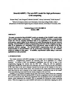
Figure 6 shows that the computed standard deviation approaches the national empirical standard deviation of confidants.
Computed vs Empirical Standard Deviation 4.5
4
3.5
#confidants
3
2.5
computed standard deviation empirical standard deviation (from th reports)
2
1.5
1
0.5
19
17
15
13
9
11
7
5
3
1
85
75
65
55
45
35
25
15
0
category slots (the left half with 5 unit increments is age, while the right half is educational level)
Figure 6: Standard Deviation Estimation and Fitting by Gradient Descent Method The above shows that more iteration is needed. The minimization of the errors of mean and standard deviation is performed at the same time and same step.
Discussion We presented a method, a gradient descent algorithm, by which the base interaction probabilities between agents having different and multiple categories could be computed so that the computed number of confidants would meet the available national average of confidants (the empirical data based on the reports). The results here are general, meaning the gradient descent algorithm described could be applied to data having many more categories. However, they are limited to the case of asymmetric interaction probabilities matrix. The asymmetric matrix could be justified on the ground that each agent perceives its own probabilities of interaction with others, while the ground-truth or real probability of interaction is hidden somewhere out there in the real world. In the field of social network analysis, Krackhardt in his exposition about trust networks shows that perception is as important as, if not more, than the reality. What one perceives determines what “reality” one finds oneself in. The same case happens in this asymmetric matrix, what probability of interaction one perceives with respect to others determines to a large degree the reality of interaction. However, in the case where we want to use the real interaction probabilities and have the means to accurately measure them, we would need to use symmetric interaction probabilities matrix. The gradient descent algorithm presented could be applied to the case of symmetric matrix with slight modifications, namely to ensure that every other row or column affected by a modified cell has the new computed number of confidants having smaller absolute errors of both mean and standard deviation with respect to the national empirical data.
Value of This Research This research represents the first step toward a general algorithm, which could take empirical data -- populationlevel data or census data -- and generate sets of different heterogeneous agents whose total behavior matches the empirical data. This matching with empirical data would make agents much more realistic than current state-of-theart. Realistic agents are essential if we are to have realism in our simulation and evaluation of organization theories based on them. The social interaction algorithm CONSTRUCT [Carley, 1990] and the agent-based epidemiological models could benefit from this research. In the field of organization theory, realistic heterogeneous agents are essential to model the reality of today workplace in more precise detail (agent-level detail) than previous work.
Limitations and Future Work This research has the following limitations: • It does not take into account the network structure surrounding an agent in determining the probability of interaction with other agents. High in-degree and out-degree agents may or may not have more confidants. This is not explored in this research. • The example is currently limited to only two categories, but could easily be expanded to much more. • Sensitivity analysis is not done. Sensitivity analysis is useful in determining which sets of agents we would like to adjust (of their interaction probabilities) first, thus making convergence of gradient descent faster. • This work is limited to only one measure: the number of confidants. Future work may extend to many more measures. • The computation of base probabilities is currently based on simple calculation. Future work may want to compare this to simulated agent approach. Simulated agent approach means we take the base probabilities of agents (with their random increments) and simulate the agents. At the end of each simulation the absolute errors are computed, and based on this, we either accept or reject the increments. The simulation would doubtlessly take much more time than simple computation, but it is interesting to see if it makes any difference. • No network data is considered. Neither network analysis is performed. Future work may want to explore this. • Current algorithm is a single-processing algorithm. Future work may look to expand this to a parallelized multi-processing algorithm.
In addition to fixing the above limitations, future work may look at: • Extending realistic agents to realistic society. Note that the addition of agents does not give us society. A society is much more complex than mere summation of agents. Society includes cultures, symbols, history, religion, technology, myth, shared meanings, and politics, and is influenced by geography and climate. Smircich described organizations as culture and shared meaning, but her analysis is limited to organizations, not society [Smircich, 1996]. • Extending agents to take into account intra- and inter-organizational networks. Power [Powell, 1990] described the network forms of organization. • Extending the knowledge of agents to include culture and culture interaction & transmission modes. • Combining heterogeneous agents with the conventional organizational/public policy planning methods. • Expand the cognition ability of an agent to include cultural cognition [Huchins, 1995].
References [Carley, 1986] Carley, Kathleen M, 1986, “Measuring Efficiency in a Garbage Model”, in J. March & R. Weissinger-Baylon (eds.), Ambiguity and Command: Organizational Perspectives on Military Decision Making, Pitman Publishers, Boston, MA. [Carley, 1990] Carley, Kathleen M, 1990, “Group stability: A socio-cognitive approach”, in E. Lawler, B. Markovsky, C. Ridgeway, H. Walker (eds.), Advances in Group Processes: Theory and Research. (pp. 144). Greenwich, CT: JAI Press. [Carley et. al., 1992] Carley, KM, et. al., 1992, “Plural-Soar: A Prolegomenon to Artificial Agents and Organizational Behevior”, in Masuch and Masimo (eds), Artificial Intelligence in Organization and Management Theory: Models of Distributed Activity, North-Holland, pp. 87-118. [Carley and Prietula, 1994] Carley, KM and Prietula MJ, Computational Organizational Theory, Lawrence Erlbaum Publishers. [Carley and Gasser, 1999] Carley, KM and Gasser L., 1999, “Computational Organizational Theory”, in Weiss, Gerhard (ed.), Distributed artificial Intelligence, MIT Press, Ch. 7. [Carley and Newell, 1994] Kathleen Carley & Allen Newell, 1994, “The Nature of the Social Agent.” Journal of Mathematical Sociology , 19(4): 221-262. [Evan, 1993] Evan, WM, Organization Theory: Research and Design, Macmillan Publishing Co. [Friedland and Alford, 1991] Friedland, R. and Alford, RR., 1991, “Bringing Society Back In”, in The New Institutionalism in Organisational Analysis. [Harrison and Carroll, 1991] Harrison, JR and Carroll GR, “Keeping the Faith: A Model of Cultural Transmission in Formal Organizations”, Admisnistrative Science Quarterly 36, pp. 552-582 [Huchins, 1995] Huchins, E, 1995, “Cultural Cognition”, in Cognition in the Wild, Ch. 9. [Levinthal, 2001] Levinthal, D., 2001, “Modeling adaptation on Rugged Landscapes”, in A. Lomi and ER. Larsen (eds), Dynamics of Organizations: Computational Modeling and Organizational Theories, MIT Press/AAAI Press. [Louis, 1980] Louis, MR, 1980, “Organizations as Culture-Bearing Milieux”, in JR Shafritz and JS Ott (eds), Classics of Organization Theory, Wadsworth Publishing Co. [Masuch and LaPotin, 1989] Masuch, M and LaPotin, P, 1989, “Beyond Garbage Cans: An AI Model of Organizational Choice”, Administrative Science quarterly, 34:38-67. [Mintzberg, 1979] Mintzberg, Henry, 1979, “The Five Basic Parts of the Organization”, in J. M. Shafritz and J. S. Ott (eds.), Classics of Organization Theory, Harcourt Brace, 1996. [Ouchi and Wilkins, 1985] Ouchi and Wilkins, “Organizational Culture”, Annual Review of Sociology, 11, pp 457-483. [Parsons, 1990] Parsons, Talcott, 1990, “Social Systems”, in The Sociology of Organizations. [Powell, 1990] Powell, WW, 1990, “Neither Market Nor Hierarchy: Network Forms of Organization”, Research in Organizational Behavior, 12, JAI Press, pp 295-336. [Prietula et. al., 1998] Prietula MJ, 1998, Simulation Organizations, AAAI / MIT Press [Prietula, 2000] Prietula, MJ, 2000, “Advice, Trust, and Gossip Among Artificial Agents”, in CASOS Conference 2000. [Roberts, 1989] Roberts, K.H., 1989, “New Challenges to Organizational Research: High Reliability Organizations”, Industrial Crisis Quarterly, 3: 111-125. [Schein, 1996] Schein, EH, 1996, “Defining Organizational Culture”, in JR Shafritz and JS Ott (eds), Classics of Organization Theory, Wadsworth Publishing Co.
[Smircich, 1996] Smircich, L., 1996, “Organizations as Shared Meaning”, in JM Shariftz and JS Ott (eds.), Classics of Organization Theory, Ch. 46.