Generating Road Network Graph with Vision-Based Unmanned Vehicle

International Journal of Undergraduate Research and Creative Activities Volume 9

February 2017

Generating Road Network Graph with VisionBased Unmanned Vehicle Henrique Yano Federal University of ABC, [email protected]

Francisco Zampirolli Federal University of ABC, [email protected]

Follow this and additional works at: http://commons.pacificu.edu/ijurca Recommended Citation Yano, Henrique and Zampirolli, Francisco (2017) "Generating Road Network Graph with Vision-Based Unmanned Vehicle," International Journal of Undergraduate Research and Creative Activities: Vol. 9, Article 2. DOI: http://dx.doi.org/10.7710/2168-0620.1083

Article 2

Generating Road Network Graph with Vision-Based Unmanned Vehicle Peer Review

This work has undergone a double-blind review by a minimum of two faculty members from institutions of higher learning from around the world. The faculty reviewers have expertise in disciplines closely related to those represented by this work. If possible, the work was also reviewed by undergraduates in collaboration with the faculty reviewers. Abstract

With the advancement of technology and its cheapness, robotic vehicles have gained a large number of applications. The spread of their use is growing also because they are getting smaller, lighter and easier to build. In this paper we present a simple and effective way to map a road network with the help of a driverless vehicle. Our approach consists of only three parts: vision-segmentation, angle variation and travelled distance. A video camera attached to a Lego® NXT Mindstorm vehicle guides it by image segmentation using Matlab® Image processing toolbox, along a road network, in which is represented by black tape over a white floor. The algorithm makes the vehicle travel all over the road memorizing main coordinates to identify all crossroads by keeping track of the travelled distance and the current angle. The crossroads and road’s end are the nodes of the graph. After several simulations have been performed, the modelling proved to be successful in that small scale approach. Consequently, there are good chances that driverless cars and UAVs also make use of the strategies to map route networks accordingly. The algorithm presented in this paper is useful when there is no localization signal such as GPS, for example, navigation on water, tunnels, inside buildings, among others. Keywords

Computer Vision, Unmanned Vehicles, Vehicle Guidance, Route Mapping. Acknowledgements

Great acknowledgments to Federal University of ABC, who gave us the necessarily support to this research.

This research article is available in International Journal of Undergraduate Research and Creative Activities: http://commons.pacificu.edu/ijurca/vol9/iss1/2

Yano and Zampirolli: Generating Graph with with Vision-Based Unmanned Vehicle

INTRODUCTION Vision-based systems consist of a sequence of digital images that enable the detection and the identification of objects. Iris and face recognition are examples of vision-based systems applied to security and private access control. Many other applications can be found in traffic control, search and rescue, border security and aerial surveillance. These tasks are already accomplished by vision-based robots, which are nowadays built with inexpensive equipment and have an easy maintenance. Several techniques to endow vehicles with vision-based control can be found in (Güzel, 2013; Bertozzi & Broggi, 1997; Tisdale, et al., 2009; Carloni, et al., 2013; Yunji, et al., 2013; Ivancsits & Lee, 2013; Lim, et al., 2012; Mahony, et al., 2012; Guillet, et al., 2014; Mcgill & Taylor, 2011). They enable object detection, path orientation and distance control. Vision-based control makes signal reception more robust than other vision guidance methods do. For instance, GPS (Global Positioning System) receives satellite signals with a considerable margin of error, besides the fact that such signals are sometimes blocked, for example, under the water, inside tunnels or inside buildings. The first mobile robot was built in the 70s in Stanford Research Institute. Another example of mobile robot, now with a video camera for navigation aid, was developed in the 80s at Carnegie Mellon University (Güzel, 2013). Other vehicles have been tested with GPS and video cameras. For example, aircraft fuselage (Tisdale, et al., 2009; Kendoul, et al., 2009), helicopters (Yunji, et al., 2013; Ivancsits & Lee, 2013), quadmotors (Carloni, et al., 2013; Ivancsits & Lee, 2013; Lim, et al., 2012; Mahony, et al., 2012; Frew, et al., 2004), road robots (Bertozzi & Broggi, 1997; Guillet, et al.,

2014; Neto, et al., 2009) and flying simulator games (Neto & Campos, 2009; Neto, et al., 2011) use Dubin’s Path Waypoints (Dubins, 1957). All these vehicles use different approaches of location and orientation methods with techniques that either focus on the odometer or on the accelerometer, or even on the GPS itself. These different approaches make unmanned vehicles over uncovered areas render different mappings. See Güzel, 2013; Bertozzi & Broggi, 1997; Tisdale, et al., 2009; Carloni, et al., 2013; Yunji, et al., 2013; Ivancsits & Lee, 2013; Lim, et al., 2012; Mahony, et al., 2012) for an overview. Some related to projects aim at a geographical image mapping that gives relevant data to agricultural activity (Guillet, 2014; Medeiros, 2008). With advanced cameras one can also plot 3D maps. In (Eisenbeiss, 2004) the author shows an example of photogrammetry, in which a helicopter was used to obtain some data from a settlement of the 13th century A.D. in Peru. By flying automatically according to predefined path points these data produced a 3D image of that settlement. In (Sibley, et al., 2010) it is possible to see a study of robot location on Mars, with an approach of sliding window filter. In (Newcombe, et al., 2011) it provides a very detailed approach to mapping techniques using a Kinect sensor for mapping of the indoor scenes. In this study it will be performed simulations with an indoor model, where one video camera attached to a robot guides it by image segmentation along a road network, represented by black tape over a white floor. Hence either GPS or any other outdoor equipment cannot be included in our tests. Therefore, we resort to mapping techniques like orientation by angle and travelled distance.

1

International Journal of Undergraduate Research and Creative Activities, Vol. 9 [2017], Art. 2

MATERIALS AND METHODS The main goal of this project is the elaboration of a strategy to automate the mapping of road networks modelled by black tape over a white floor (Figure 1). Automation is done by an unmanned vehicle that travels across the network and is guided only through image measurements. In this case will be used the LEGO NXT Mindstorm vehicle (Figure 1) that drives through the path according to one Matlab® program, transmitted via Bluetooth. The program ensures that our vehicle will never come off the trail, and also its coordinates will be stored continuously. Moreover, the program identifies all the coordinates that represent a crossroad. The crossroads and the road’s end are the nodes (or vertices) of the graph, where the edges are pairs of nodes, represented by (x, y).

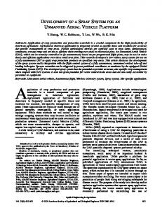
vehicle must proceed with the appropriate command that keeps the next road stretch within the camera range. For this purpose, we use Mathematical Morphology (Corke, 2005; Gonzalez & Woods, 2007; Serra, 1982; Serra, 1988) to analyze the image and then choose a suitable command that will be executed by the steering wheel and the motor. This algorithm uses the function IMGsegm, which give orders to move according to the image of the tape pieces and their arrangement. Figure 2 shows some examples of images and their corresponding commands.

Figure 2. Images of “crossroad” (left), “straight route” (middle) and “turn left” (right).

In order to choose the suitable command, the image is submitted to a segmentation process that follows a sequence of functions contained in the Matlab® Image processing toolbox. Firstly, the image is converted to binary format and fits into a square of L x L pixels that will be called IMG. Then a square of (L-30) x (L30) pixels is removed from the center of IMG. What remains are just boundary objects, as illustrated in Figure 3. Figure 1. Vehicle LEGO NXT over a prototype of road network.

A. Segmentation of Road Images The camera calibration is an important activity (Keivan & Sibley, 2015). In this paper, a low-cost camera (2MP and f4.8mm) was fixed on the robot to 8 cm from the floor, (Figures 1 and 10). The black tape attached over a white floor has 8mm wide. According to each captured image the

http://commons.pacificu.edu/ijurca/vol9/iss1/2 DOI: http://dx.doi.org/10.7710/2168-0620.1083

Figure 3. Image submitted to the segmentation process.

In Figure 3, right side, there are two white components, in which aiming from the bottom one to the other one determines the

2

Yano and Zampirolli: Generating Graph with with Vision-Based Unmanned Vehicle

direction of the movement. Moreover, the inclination between these two components determines the intensity of the movement. We calibrate the robot rotors using a constant time with the command "pause" the Matlab® as value 1.5 milliseconds. So we do capture a frame, processing the image and the PC sends a command via Bluetooth for the robot rotors, then wait for these 1.5 milliseconds. This type of robot movement is detailed in (Yano & Zampirolli, 2013). Function IMGsegm; Receive image imgcaptured; imgSegment=Segment(imgcaptured); Degree=Orientation(imgcaptured); Switch imgSegment Case {“straight route”} Order = “go forward”; Case {“road end”} Order = “road end”; Case {“left route”} Order = “turn left”; Case {“right route”} Order = “turn right”; Case {“crossroad”} Order = “crossroad”;

The cases of three or more components (when the robot finds a crossroad for example, having more than one option to follow the road network) are treated by pairwise analyses and it will be explained ahead. B. The Function Map Our function called Map was implemented with the same logic used by soldiers and scouts when they guide themselves in jungles and fields (Department of The Army, 2007). For that, one only needs to track their travelled distance and to use a compass. They are instructed to walk a distance in the direction of a certain angle referenced by the North magnetic pole. When they reach the correct point, a new distance has to be walked along a new direction. This procedure is simple to

follow and discards any elaborate equipment. For this reason, we chose it in order to elaborate our algorithm. The two important data (angle and distance) are obtained by means of image segmentation. Our vehicle starts at a point given by (d1, α1) in polar coordinates regarding a fixed origin. If it turns and then goes to another stop this is counted as (d2, α2) with respect to (d1, α1). By repeating the process, we shall have (d3, α3) regarding (d2, α2) and so forth (Margolis & Yasui, 1995).

Figure 4. Example of mapping with angles and distances.

The example shown in Figure 4 indicates two positions given by (x1, y1) and (x2, y2) in rectangular coordinates. Of course, (x1, y1) = (d1*cos(α1), d1*sin(α1)) and (x2, y2) = (x1, y1) + (d2*cos(α2), d2*sin(α2)). The general recursive formula is (xn, yn) = (xn-1, yn-1) + (dn*cos(αn), dn*sin(αn)) for a natural number n ≥ 2. C. Vehicle Movement Whenever the function IMGsegm gives an order the function LEGO_Movement reads the order and activates the steering wheel and the motors accordingly. This algorithm not only controls the motors but also records the vehicle coordinates and its orientation. The intensity of the motor rotation is defined by the route angle, namely the

3

International Journal of Undergraduate Research and Creative Activities, Vol. 9 [2017], Art. 2

variable called Degree, so that it works like a steering wheel. Large angle variations thrust the rotation of the whole vehicle. We remark that in the function LEGO_Movement there is a special function called Map, which is invoked whenever Order is equal to “crossroad” (when the robot finds a fork or a crossroad, having more than one option to follow the road network). Those two lines of source code do not define the movement itself, which will be in fact established by the new string stored in Order and the Switch command that follows in the sequel. Function LEGO_Movement; Test Motors, Connection and Camera ANG=0; j=1; X[0]=0; Y[0]=0; % used on Map While (non-stop) Camera capture imgcaptured; Order = IMGsegm(imgcaptured); If Order == “crossroad” Order = Map(imgcaptured); Switch Order Case { “road end” } Invert vehicle direction; ANG = ANG + 180º Case { “turn right” } Move vehicle to right; ANG = ANG - Degree; Case { “turn left” } Move vehicle to left; ANG = ANG + Degree; Case { “go forward” } Move vehicle forward; X[j] = X[j-1] + d*sin(ANG); Y[j] = Y[j-1] + d*cos(ANG);

The function Map records the main road coordinates and also makes the appropriate decision on which direction will be taken whenever the vehicle arrives at a crossroad. For example, when choosing a direction with the lowest weight stored in an adjacency matrix, this will be exemplified in the next section. The main goal of this paper is the implementation of the function Map, which defines a graph in which the vertices are the centroids of each crossroad and of each road

http://commons.pacificu.edu/ijurca/vol9/iss1/2 DOI: http://dx.doi.org/10.7710/2168-0620.1083

end. In the graph edges represent the road stretches that connect these centroids. D. The Function of Generating Road Network Graph The following code is the algorithm of the function Map: Function Map; imgLabel = bwlabel(imgcaptured); regioprops(imgLabel, “centroids”); crossroad = “unknown”; For i = 1 to size(CX) If {X(end),Y(end)}≈{CX(i),CY(i)} crossroad = “known”; stopFor; Switch crossroad Case { “unknown” } {CX(j),CY(j)}={X(end),Y(end)}; For h=1 to Ne-1 CA(j,h) = ANG + angles(Ne) A = random h; Order = direction(CA(j,A)); CA(j,A) = 0; j = j + 1; Case { “known” } For h = 1 to Ne If CA(i,h) ~= 0; StopFor; Order = direction(CA(i,h)) CA(i,h) = 0;

The mapping coordinates recorded by the function LEGO_Movement are used to distinguish crossroads between tracked and untracked. The tracked crossroads are stored in the coordinate vector {CX, CY}. When the vehicle arrives at a crossroad its current coordinates (X(end), Y(end)) are compared with each element in {CX, CY}. If sufficiently close coordinate numbers are found this means that the crossroad has already been tracked. Otherwise it has not yet. In the latter case both the new coordinates and the incident paths are recorded in CA. Afterwards the program chooses one of the paths at random for the vehicle to move on.

4

Yano and Zampirolli: Generating Graph with with Vision-Based Unmanned Vehicle

Figure 5 shows an example of a crossroad segmentation in which the final image shows four objects. Each one indicates the possible paths by means of the angles that it makes with the other objects.

segmentation process explained beforehand (Figure 3). The relative angles are listed in the vector CA, of which columns represent the crossroad counter and each line shows the incident paths of the crossroad. If the path has already been tracked its value is set as zero. If the crossroad is tracked, it means that CA has recorded the incident paths. So the order is defined by the first non-zero direction element.

Figure 5. Segmentation process of a crossroad image.

This procedure is implemented as the function regionprops, which analyses each object and locates its centroid regarding the image coordinates. The function bwlabel counts the number of isolated objects in the binary image. This number is stored in the vector Ne. For more information about these Matlab functions see www.mathworks.com/ products/image. The incident paths of a crossroad are identified by their relative angles, as illustrated in Figure 6.

EXPERIMENTAL A. First Experiment In this first experiment to create a graph from the robot navigation in a row simulating a road network, it will be considered, in simplified form, only two images. The first image has a vertical line, or “straight route”. The second image is a “crossroad”. These images after segmentation are shown in Figure 7 (as the images used in the experiments have high contrast, this segmentation used a threshold 80 and a morphological opening with a disk of radius 20 pixels in one of the bands RGB).

Figure 6. Distinguishing incident paths of a crossroad.

The relative angles are defined as the sum of the current orientation with each necessary turning angle. In this way the paths are correctly recognized again no matter from which direction the vehicle arrives. In order to find the turning angle, the crossroad image is submitted to the same

Figure 7. Images “straight route” (left) and “crossroad” (right).

These images of Figure 7 are exchanged, as follows, as if the robot were "seeing" the image of the “straight route” into two consecutive frames, and the third

5

International Journal of Undergraduate Research and Creative Activities, Vol. 9 [2017], Art. 2

frame is an image of the “crossroad”. The starting point is the image of the vertical path. As a validation of movements, the simulator initially returns the following variables: ANG = [0 X = [0 Y = [0 GO AHEAD

-0.0058] -0.0233] 3.9999]

The angle -0.0058 is the vertical slope of the line shown in Figure 7 (left), using the orientation attribute of regionprops function of Matlab. The X and Y values were calculated as follows: X = [X Y = [Y

X(end) + d*sin(ANG(end))] Y(end) + d*cos(ANG(end))]

where d = 4. This value should be calibrated, with the movements of the robot rotors. The next frame to be processed is also the same “straight route” and the simulator returns: ANG = [0 X = [0 Y = [0 GO AHEAD

-0.0058 -0.0233 3.9999

-0.0117] -0.0699] 7.9996]

The angle -0.0117 is calculated with the difference (-0.0117=-0.0058-0.0058) of the two vertical slopes of the line shown in Figure 7 (left). The same occurs in X (0.0699=-0.0233-0.0466) and in Y (7.9996=3.9999+3.9997). The next frame was a “crossroad”, we now have the following variables: ### CROSSROAD ### FIRST NODE FOUND ANG_actual = 0 ### CROSSROAD UNKNOWN ### CX = [0] CY = [0] CANG = [-1.527 0.0626 -0.0329 ANG(end) = 1.5338 Node_preview = 1 TURN RIGHT

1.5338]

In this first "crossroad", we define the first graph node in the coordinate (0,0) of the Cartesian Plane, we have 4 possible directions, with the angles stored in CA. In this first experiment, we will consider always the 4 angle, i.e., the robot will always turn to the right. This angle is also stored in ANG. The next frame is the "straight route", and we have the following variables: ANG = [1.5338 X = [0 Y = [0 GO AHEAD

1.5279] 3.9963] 0.1714]

Again, another frame "straight route", we now have the following variables: ANG = [1.5338 X = [0 Y = [0 GO AHEAD

1.5279 3.9963 0.1714

1.5221] 7.9916] 0.3660]

Now another "crossroad" will be processed with the following output: ### CROSSROAD ### ANG_actual = 1.5221 ANG(end) = 1.5221 CX = 7.9916 CY = 0.3660 ### CROSSROAD UNKNOWN ### CX = [0 7.9916] CY = [0 0.3660] CA = -1.5273 0.0626 -0.0329 -1.5273 0.0626 -0.0329 ANG(end) = 3.0559

1.5338 1.5338

MatrixAdj = 0 1 0 0 0 0 0 0 0 0

0 0 0 0 0 0 0 0 0 0

0 0 0 0 0 0 0 0 0 0

0 0 0 0 0 0 0 0 0 0

0 0 0 0 0 0 0 0 0 0

0 0 0 0 0 0 0 0 0 0

0 0 0 0 0 0 0 0 0 0

0 0 0 0 0 0 0 0 0 0

0 0 0 0 0 0 0 0 0 0

0 0 0 0 0 0 0 0 0 0

Node_preview = 2 countVERT = 3 TURN RIGHT

In the latter process, the simulator calculates the second node of the graph. So,

http://commons.pacificu.edu/ijurca/vol9/iss1/2 DOI: http://dx.doi.org/10.7710/2168-0620.1083

6

Yano and Zampirolli: Generating Graph with with Vision-Based Unmanned Vehicle

we can now use an adjacency matrix to store the neighbourhood of each node of the graph, see the contents of the variable MatrixAdj where node 1 is adjacent to the node 2 (and vice versa). Figure 8 shows this graph with two nodes already processed, one at position (0, 0) and the other at (7.9916, 0.3660), calculated by taking the last element of each coordinate, or CX = X(end) = 7.9916 and CY = Y(end) = 0.3660.

The adjacency matrix after six processing of "crossroad" is shown below: MatrixAdj = 0 2 0 0 0 0 0 0 0 0

0 0 1 0 0 0 0 0 0 0

0 0 0 1 0 0 0 0 0 0

1 0 0 0 0 0 0 0 0 0

0 0 0 0 0 0 0 0 0 0

0 0 0 0 0 0 0 0 0 0

0 0 0 0 0 0 0 0 0 0

0 0 0 0 0 0 0 0 0 0

0 0 0 0 0 0 0 0 0 0

0 0 0 0 0 0 0 0 0 0

B. Second Experiment In this second experiment, the robot will be shown driving through a simulation of a road network in blocks, steering always to the right when a "crossroad" is found. See Figure 10.

Figure 8. Graph with 2 nodes in (0, 0) and (7.9916, 0.3660).

This processing (two frames "straight route" and one frame "crossroad") are repeated indefinitely. Considering more three nodes of the graph, we will have an overlap of nodes (within a margin of error), so we do not account for new nodes of the graph, as shown in Figure 9. Figure 10. Image with the robot in the road.

The graph produced by this second experiment is shown in Figure 11. In this case it was used to scrolling constant d=1. Images, videos and data produced in experiments of this paper are available at http://vision.ufabc.edu.br/RobotRoad.

Figure 9. Graph with 4 nodes.

7

International Journal of Undergraduate Research and Creative Activities, Vol. 9 [2017], Art. 2

Figure 11. Another graph with 4 nodes, now with the robot in the road.

DISCUSSION The weights in the adjacency matrix indicate how often the robot travelled over the same edge. The adjacency matrixes used in the experiments had considered graphs of up to 10 nodes, the higher the number of "crossroad" in the road network, the bigger must be the adjacency matrix. After several iterations of the robot driving through the same edge (consequently, same pairs of nodes), it is recommended to make an adjustment of the coordinates of the nodes, for example, by averaging the coordinates in several visits in the same "crossroad". In the performed experiments in this paper, always when the robot arrives in a "crossroad" it will turn the rightmost edge or leftmost edge, or it will choose a random edge. With little change in the algorithm, it can be avoided the robot walking the edges which it had already visited. Thus, the robot will walk on all edges and on all nodes of the graph (connected).

CONCLUSION In this paper it was created an algorithm to identify important coordinates

http://commons.pacificu.edu/ijurca/vol9/iss1/2 DOI: http://dx.doi.org/10.7710/2168-0620.1083

on a road by guiding an unmanned vehicle using image processing. The code written in Matlab sends orders to a LEGO NXT vehicle with an attached camera, from which an image segmentation algorithm determines the movement. This algorithm ensures that the road is kept within the camera range while it travels along the road network, and another algorithm memorizes the coordinates of the crossroads to decide which way the vehicle has to take, ensuring that not a single path will be left untracked. After having implemented these algorithms, several tests were performed. The vehicle moved according to the expected performance and all the crossroad coordinates were recorded correctly. Therefore, we conclude that our visionbased strategy and the LEGO NXT kit have both succeeded in the indoor modelling. Furthermore, an important extension of our map creation strategy is another algorithm adapted to GPS. This way the vehicle could travel much larger distances. In future works we intend to apply these results to other vehicles, specially to medium range aerial vehicles that fly over streets, rivers or marks on the ground, and use the aforementioned image processing algorithm.

REFERENCES Bertozzi, M. and Broggi, A. (1997). Visionbased vehicle guidance. Computer, Vol. 30, no. 7, 49-55. Carloni, R., et al. (2013). Robot Vision: Obstacle-Avoidance Techniques for Unmanned Aerial Vehicles. Robotics & Automation Magazine, IEEE, Vol. 20, no. 4, 22-31. Corke, P. I. (2005). The Machine Vision Toolbox: a MATLAB toolbox for vision and vision-based control. Robotics &

8

Yano and Zampirolli: Generating Graph with with Vision-Based Unmanned Vehicle

Automation Magazine, IEEE, Vol. 12, no. 4, 16-25. Department of The Army, (2007). The Soldier's Guide: The Complete Guide to U.S. Army Traditions, Training, Duties, and Responsibilities. Skyhorse Publishing. Dubins, L. E. (1957). On curves of minimal length with a constraint on average curvature and with prescribed initial and terminal positions and tangent. American Journal of Mathematics, Vol. 79, 497516. Eisenbeiss, H. (2004). A Mini Unmanned Aerial Vehicle (UAV): System Overview and Image Acquisition. International Workshop on Processing and Visualization Using HighResolution Imagery, Pitsaulok, Thailand. Frew, E., et al. (2004). Vision base droadfollowing using a small autonomous aircraft. Aerospace Conference. Proceedings, IEEE 5: 3006-3015. Gonzalez, R. C. and Woods, R. E. (2007). Digital Image Processing. Prentice Hall; 3 ed. Guillet, A., el al. (2014). Adaptable Robot Formation Control: Adaptive and Predictive Formation Control of Autonomous Vehicles. Robotics & Automation Magazine, IEEE, Vol. 21, no. 1, 28-39. Güzel, M. S. (2013). Autonomous vehicle navigation using vision and maples strategies: a survey. Advances in Mechanical Engineering. Ivancsits, C. and Lee, M. R. (2013). Visual navigation system for small unmanned aerial vehicles. Sensor Review, Vol. 33 no. 3, 267-291. Keivan, N. and Sibley, G. (2015). Online SLAM with any-time self-calibration and automatic change detection. Robotics and Automation (ICRA), IEEE International Conference on. IEEE, 2015.

Kendoul, F., et al. (2009). An adaptive vision-based autopilot for mini flying machines guidance, navigation and control. Autonomous Robots, Vol. 27, no. 3, 165-188. Lim, H., et al. (2012). Build Your Own Quadrotor: Open-Source Projects on Unmanned Aerial Vehicles. Robotics & Automation Magazine, IEEE, Vol. 19, no. 3, 33-45. Mahony, R., et al. (2012). Multirotor Aerial Vehicles: Modeling, Estimation, and Control of Quadrotor. Robotics & Automation Magazine, IEEE, Vol. 19, no. 3, 20-32. Margolis, D. and Yasui, Y. (1995). Automatic lateral guidance control system. U.S. Patent No. 5,390,118. Mcgill, K. and Taylor, S. (2011). Robot algorithms for localization of multiple emission sources. ACM Computer Survey, Vol. 43, no. 3, Article 15. Medeiros, F. A., et al. (2008). On the use of unmanned aerial vehicle for acquisition of georrefecend image data. Ciência Rural, Vol. 38, no. 8, 2375-2378. Neto, A. A. and Campos, M. F. M. (2009). On the Generation of Feasible Paths for Aerial Robots with Limited Climb Angle. International Conference on Robotics and Automation. Kobe, Japan. Proceedings. IEEE 5: 2872-2877. Neto, A. A., et al. (2009). Adaptive complementary filtering algorithm for mobile robot localization. Journal of the Brazilian Computer Society, Vol. 15, no. 3. Neto, A. A., et al. (2011). Nonholonomic Path Planning Optimization for Dubins’ Vehicles. International Conference on Robotics and Automation. Shanghai, China. IEEE 4208 –4213. Newcombe, R. A., et al. (2011). KinectFusion: Real-time dense surface mapping and tracking. Mixed and

9

International Journal of Undergraduate Research and Creative Activities, Vol. 9 [2017], Art. 2

augmented reality (ISMAR)10th IEEE international symposium on. IEEE. Serra, J. (1982). Image analysis and mathematical morphology. London: Academic Press. Serra, J. (1988). Image analysis and mathematical morphology – Vol. II: theoretical advances. London: Academic Press. Sibley, G., et al. (2010). Sliding window filter with application to planetary landing. Journal of Field Robotics, Vol. 27, no. 5, 587-608. Tisdale, J. et al. (2009). Autonomous UAV path planning and estimation. Robotics & Automation Magazine, IEEE, Vol.16, no. 2, 35-42. Yano, H. H. and Zampirolli, F. A. (2013). Image processing in unmanned vehicles: Identification of cases of a road to help vehicle guidance. IX Workshop de Visão Computacional. Yunji, Z., et al. (2013). Improved VisionBased Algorithm for Unmanned Aerial Vehicles Autonomous Landing. Journal of Multimedia, Vol. 8, no. 2, 90-97.

http://commons.pacificu.edu/ijurca/vol9/iss1/2 DOI: http://dx.doi.org/10.7710/2168-0620.1083

10