Generating War Game Strategies Using A Genetic Algorithm Timothy E. Revello
Robert McCartney
Computer Science & Engineering Department University of Connecticut Storrs, CT 06269-3155
[email protected]
Computer Science & Engineering Department University of Connecticut Storrs, CT 06269-3155
[email protected]
Abstract - Unlike most games which have fixed rules, the rules for war games can contain uncertainty. This uncertainty makes war games difficult to address with methods typically used for playing games by machine. The characteristics of war games match well with the domain for which genetic algorithms are effective. In this paper we explore the use of genetic algorithms for generating war game strategies.
1 INTRODUCTION Many problems of interest take the form of games. Gaming is used extensively by the military, the diplomatic corps, and business to assist in planning for future courses of action and decision making. Games are often used in research as a venue for the development of problem solving techniques. Studying the solutions to games, even simple ones, is of interest since the lessons learned can be applied to real world situations. Game play has been a topic of research in computational science for some time. Problems like the eight or fifteen tile puzzles, tic-tac-toe, and the Tower Of Hanoi have often been used. These are all fairly simple in nature. More complex games like checkers and chess have also been addressed. In these games, a subproblem such as an end game strategy may be the topic of an investigation as well as the full game itself. War gaming has been practiced in one form or another since before the beginning of recorded history. Currently, it is widely used in various military organizations around the world for both training and research. A comprehensive treatment of war gaming can be found in [1]. Included is an extensive review of the history and development of the subject. Some issues and challenges in contemporary war gaming are discussed in [2]-[4]. One of the challenges currently faced is to better address uncertainty, which is an important factor in actual conflicts. Games in general, as well as war games, can contain uncertainty. One type of uncertainty has to do with variables working inside of the framework of the rules of the game. There is uncertainty in what moves the opposition will make, what the dice roll will be, or what card will be turned up. This first type of uncertainty can be found in war games as well as many other types of games. A second type of uncertainty, which is found in war games but not most other games, has to do with uncertainty in the rules of the game themselves. In real world situations such as those modeled by war games, the specifics of what is required to win are generally not known. As an example, it is not known in advance how much punishment a military opponent will accept before surrendering. They may be
0-7803-7282-4/02/$10.00 ©2002 IEEE
willing to fight to the end. They may be only willing to tolerate a certain level of economic and military damage before conceding the battle in hopes of ensuring regime survival. Uncertainty in the rules complicates the task of determining good strategies for playing war games. In the field of artificial intelligence, methods have been developed for playing a variety of games by machine. For a game like the eight or fifteen tile puzzles where there is no active competitor, the problem can be represented using a state space tree. Heuristic search techniques like the A* algorithm are used to search the tree for a goal node. An evaluation function is used to estimate the distance from the current node to a goal node [5]. This approach is difficult to apply to a war game with uncertain rules. The state space becomes ill defined since the location of the goal nodes are not known. Estimating the distance to a goal node in order to assess which of several paths to take is also made difficult. In a war game there may be more than one potential goal. Reaching any one of the goals causes the game to be won. The values of these goals change each time the game is played. In games like checkers that have two players, game tree representations have been used in playing by machine. The game tree is searched using a technique like the minimax algorithm. Evaluation functions are used to estimate the value of a position resulting from moves and opponent’s countermoves [5]. Most efforts to play checkers and similar games by computer also involve the accumulation of expert knowledge and the application of powerful computing assets for conducting extensive searches. The most successful computer checkers program devised to date is Chinook [6]. This massive multi-year effort to accumulate as much checker knowledge as possible along with the use of powerful computing assets has produced a world class checker playing program and has defeated the human world checkers champion in match play. Average minimum search depth for a given move is 21 ply. The program has access to an extensive database of opening moves from previous championship play as well as analysis of previously unknown openings. There is an endgame database containing all approximately 440,000,000,000 possibilities given eight or fewer remaining pieces. A very similar approach was used to create the Deep Blue chess program which defeated the world champion Gary Kasparov in a six game exhibition match in 1997 [7]-[8]. Given the nature of war games, this approach would also be difficult to apply. The extensive searches conducted and databases used are all based on the game structure and rules being fixed. In war games, the rules are uncertain and
change each time a game is played. In addition, in professional war gaming, games are customized to situations of interest. A game is designed, played, and the results are analyzed. Though variants or similar situations may be studied, the exact same game may never be played again. In this paper we present results from an investigation of the use of genetic algorithms (GAs) to generate strategies for war games with uncertain rules. The general topic of evolutionary computation methods and strategy and tactics in warfare related problems is discussed in [9]-[10]. GAs are effective at solving complex problems where the state space has many local maxima and minima, discontinuities, and noise [11]. This domain matches well with the characteristics of war games. The remainder of the paper is formatted as follows. In section 2 a description of the problem addressed in the investigation and the approach used to solve it is given. Sections 3 and 4 describe the GA configurations and fitness functions used respectively. In section 5, experimental results obtained are described. A brief comparison of strategies developed using a GA to examples from military history is included. In section 6 a summary of the main points is given. 2 PROBLEM DESCRIPTION AND APPROACH The use of a GA for generating war game strategies is explored using a naval blockade scenario as a tool. In the scenario, Red is the opponent and Blue is the player for which a strategy is being determined. The goal of the game is for Blue to break a blockade imposed by Red. The number and type of ships for Blue to use and their disposition as a function of time must be determined. Red’s forces and strategy are fixed. Costs for Blue to purchase ships as well as costs for ships lost during the conflict are accounted for. Naval forces are modeled using a time step simulation. Performance of sensor and weapons systems is determined probabilistically. There are multiple possible criteria by which the game can be won. Each criterion has a range of values. The threshold value needed to achieve victory using a given criterion during a trial is selected randomly from within the range. There are eight ship types used in the game. These are listed in figure 1 along with their relative costs and the symbol used to represent them. The Red naval force is fixed and only uses patrol craft, diesel submarines, and destroyers. The composition of the Blue naval force varies during the evolution of solutions and can include any of the eight ship types. For each Blue and Red ship type, a table of probabilities describes detection and attack performance versus opposition ships. Relative capability for similar types of ships is in the same order as their costs, though not proportional. Nuclear submarines are more capable than diesel submarines, destroyers are more capable than frigates which are more capable than patrol craft, and aircraft carriers are more capable than escort carriers.
0-7803-7282-4/02/$10.00 ©2002 IEEE
type of ship
relative cost
diesel submarine nuclear submarine patrol craft frigate destroyer missile defense ship escort carrier aircraft carrier
0.5 2.5 0.1 0.4 1.0 1.0 3.0 5.0
symbol SS SSN PTG FFG DDG TBMD CVE CV
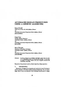
Figure 1 Figure 2 is a depiction of the game board. An inhabited island referred to as White, whose ownership is contested, lies off the coast of Red. Red has declared a blockade and placed naval forces around White. The Red forces are placed in each of the eight areas as shown in figure 2. These forces are deployed according to a predetermined strategy and do not change position. In addition to naval forces, Red has a constant land based attack capability. Red land based air forces can strike Blue surface targets in any area. The probability of a successful attack is reduced if there is a Blue aircraft or escort carrier in the area being attacked. Land based antiship cruise missile (ASCM) forces can strike Blue surface ship targets in areas 2 through 6. The effectiveness of land based forces varies with the type of Blue ship attacked. Red Coast Area 5
Area 4
Area 3
10 Red PTGs
20 Red PTGs
10 Red PTGs
Area 6 5 Red DDGs
Area 2 White 5 Red DDGs
Area 7
Area 8
Area 1
3 Red SSs
3 Red SSs
3 Red SSs
Blue Entry Points
Figure 2 Initially there are no Blue naval forces in any of the eight areas. Due to navigation constraints, Blue forces enter in either area 1 or 7. Once they enter they can move between areas but can not leave the game. Blue has up to 14 time steps to break the blockade and restore sea access to White. Blue forces can enter the board on any time step. During
each time step each Blue or Red platform has the opportunity to detect and attack opposing platforms. Two opposing ships must be in the same area before an engagement can occur. Selection of targets is done randomly from all opposing forces in the area. A Red air attack and a Red ASCM attack are also conducted in each appropriate area during each time step. A single Blue target is selected randomly during each attack. There are several criteria by which Blue can win. These are listed in figure 3. Some or all of the criteria may be used depending on the experiment being conducted. Threshold values for the quantities x in figure 3 are varied from trial to trial by selecting randomly from within some given range. This introduces uncertainty analogous to that encountered in two sided games or actual situations. Ranges of values used in the various experiments are given in the next section of the paper. A trial ends when one of the Blue criteria for victory has been satisfied or after 14 times steps or if Red wins. Red can win by destroying a given percentage of Blue forces or a given percentage of the total value of Blue forces.
The Blue force composition and disposition versus time evolves under the control of the GA. Crossover, mutation, stochastic remainder sampling without replacement, and linear scaling of the fitness function are used in the GA [12]. Two parents are selected to produce two offspring using a probability of crossover of 1.0. The probability of mutation is 0.001 for each bit in an offspring. A population size of 30 individuals is used to generate 30 offspring in each generation. Average performance for an individual in a generation is estimated using the results from 100 trials. Experiments were conducted using two different methods for estimating the average performance of an individual. These are described in the next section of the paper. Experiments are run out to 5000 generations. All individuals in the initial generation are created using random selection of bit values for each binary string. Experiments were conducted with and without elitism. The elitism scheme replaces a randomly chosen individual from the new generation with the best performing individual from the previous generation. 4 FITNESS FUNCTION
Establish air supremacy: keep 2 TBMD ships and (2 CVs or 4 CVEs) in any of the 8 areas for x consecutive time steps. Sink x % of the number of Red ships. Sink ships totaling x % of the total value of all Red ships. Demonstrate overwhelming sea control: sink x % of the Red ships in the area 4 strait. Sink the Red command ship which can be identified and is operating in either area 2 or 6.
Figure 3 3 GA CONFIGURATION The Blue force is encoded as a binary string so that it can evolve under GA control. This encoding uses a concatenation of a number of short, meaningful blocks. The encoding developed is 396 bits long, consisting of 12 groups of 33 bits each. Each group of 33 bits represents a task or ship group. The Blue force consists of up to 12 task groups. Task groups move independently without considering how other groups are moving. Each task group can have up to three ships, all of which are the same type. In a group, bits 1 through 3 designate the type of ships in the group. Bits 4 and 5 designate the number of ships in the group which ranges from 0 to 3. Bits 6 through 33 are used to designate the movement of the group in each of the 14 possible time steps. There are 14 pairs of bits, one of which indicates whether the group moves in a given time step and the other which indicates direction. Blue ships must enter in either area 1 (right side of the board) or 7 (left side of the board). Once on the board a ship can stay in its area or move to an area either to its left or to its right.
0-7803-7282-4/02/$10.00 ©2002 IEEE
The fitness function used during the investigation is shown in equation 1. It contains both cost and benefit terms and follows the form developed in [13]. In [13] it was demonstrated that including cost terms as well as benefit terms reduced the complexity of solutions developed as well as improved performance. In this investigation initial experiments were conducted with and without cost terms. Using no costs yielded solutions which reached the goal of achieving victory in all 100 trials but that were not well formed. They tended to be complex and used many times the amount of resources used when costs were applied. Well formed solutions that reached the goal were developed using the cost terms. Using the cost terms also resulted in the reduction of complexity in the solution. fitness = benefit - (Blue force cost * (benefit/max. poss. benefit) * weight_force) - (game time cost * (benefit/max. poss. benefit) (1) * weight_time)
The three main components of equation 1 are a benefit term, a term for the cost of the Blue force, and a term for the amount of time used to reach a solution. In the benefit term, the more progress that is made towards the goal, the more credit that is given. It is also desirable for the Blue force to be efficient in terms of ships used and ships lost as well as the amount of time it takes to achieve the progress that is made towards the goal. The cost terms contain dynamically scaled weights which increase the importance of efficiency the farther the Blue force is able to progress towards the goal. Benefit is the percentage progress made towards the goal of achieving victory in all the trials and has a maximum value of 100. Maximum possible benefit is simply 100 percent.
The benefit term in equation 1 was computed using one of two different methods, depending on the experiment. The first method, referred to as the criterion method, uses calculations of the progress towards the various criteria for victory. For each criterion the percentage progress made towards its threshold value is computed for each trial. An average for each criterion is then calculated. The criterion with the highest value is chosen and its value is multiplied by 100. The values from the other criteria are averaged and the result is added to the result of the previous operation with the sum not to exceed 100. Small contributions from these criteria can still be important since linear scaling of scores is used during mate selection for each generation. The second method, referred to as the count method, looks only at the percentage of trials out of the 100 where victory was achieved. For an individual trial no credit is given for partial progress towards the criteria thresholds. Any combination of criteria can be used in reaching the goal of achieving a win in all trials. In some cases the thresholds for victory are met in the same time step in a trial for more than one criterion. This is still scored as a single victory. Blue force cost and game time cost are both computed as percentages of their maximum possible values. In determining Blue force cost, costs are assessed for purchasing the ships used as well as for replacing any ships lost. The total cost for ships is then divided by the maximum ship cost to get the Blue force cost. The maximum ship cost is 72 times the cost of the most expensive ship. The maximum number of ships that can be part of the Blue force is 36 and each ship can be purchased as well as lost. Game time cost is the average number of time steps a trial took to complete divided by the maximum possible number of time steps. The force and time weights allow the user to designate the relative importance of the two cost terms. Equation 1 yields different ratios of costs and benefits during different stages of the evolution of the solution. During the early stages, cost is emphasized less and progress towards the goal is rewarded. This approach does not overly restrict the exploration of the solution space during the initial stages of development of potential solutions. In the later stages of the evolution, once the goal has been reached improvements in ship costs and execution efficiency are emphasized more. 5 RESULTS A series of experiments was conducted during the investigation using various combinations of conditions. A variety of criteria thresholds and cost weights were used. For each combination of thresholds and weights, experiments were conducted with and without elitism using both the criterion and count methods for calculating the benefit term. The results showed that the most robust configuration was the use of elitism with the count method. This had performance better than or equal to that of the
0-7803-7282-4/02/$10.00 ©2002 IEEE
other three configurations in almost all cases. Regardless of experiment conditions, the GA methodology used was able to generate strategies that reached the goal of achieving victory in all 100 trials in every experiment conducted. The strategies developed and the Blue forces used varied with problem set up. In the following, results are shown for three experiments where either cost weight or victory criterion was varied. The results demonstrate several different strategies generated for game play. These strategies contain some similarities as well as significant differences produced by varying the experiment conditions. The victory criteria and cost weights used are shown in figure 4. During each trial, the values for the various criteria for achieving victory for both the Blue and Red sides are chosen from within the given ranges. Selection within the range is made randomly using a uniform distribution. The victory criteria are those previously described in figure 2. At the bottom of figure 4 are the weights used for the cost terms in the evaluation function. The Red command ship criterion is used only in experiment M1. In this criterion, either area 2 or 6 is randomly selected with a 50 percent probability at the beginning of each trial. Blue can win by sinking one Red ship in the area selected. The scenario modeled is that the Red force commander is at sea in one of two operating areas directing the battle. The command ship is identifiable and if sunk, the Red force will be thrown into disarray and will withdraw. experiment: Blue victory criteria air supremacy (days) number Red ships sunk (%) value Red ships sunk (%) Red ships sunk, strait (%) Red command ship sunk Red victory criteria number Blue ships sunk (%) value Blue ships sunk (%) evaluation function Blue force cost weight game time cost weight
V1
V4
M1
5-12 .2-.5 .2-.5 .2-.5 n/a
5-12 .2-.5 .2-.5 .2-.5 n/a
5-12 .2-.5 .2-.5 .2-.5 yes
.2-.35 .2-.35 .2-.35 .2-.35 .2-.35 .2-.35 8 16
8 0
8 0
Figure 4 In the results that follow, the score listed for an experiment is the best score achieved by an individual during the 5000 generations. In estimating the score for an individual, there is some variability involved. Conditions for achieving victory as well as performance of platform sensors and weapon systems are determined probabilistically. Differences between estimates of score for an individual could be several points. The difference varied with strategy and how close it was to reaching the goal. The best strategies are robust and have less variability. Strategies described in the following had stable performance and were not the product of a single set of fortunate probabilistic draws. The population had stabilized
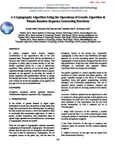
around the strategy, though not converging due to the variability involved in the game. In experiment V1, the best score achieved by an individual was 95.97. Blue achieved victory in all 100 trials. The value of Red sunk ships criterion was satisfied in all 100 trials and the number of Red ships sunk criterion was satisfied in 1. Average number of time steps in a trial was 2.92. The Blue force consisted of 36 ships. Total cost to purchase the Blue force was 28.8. On average, 2.85 Blue ships were lost during a trial with a total value of 2.49. The strategy used by Blue is demonstrated in figure 5. It shows the positions of the Blue force ships during each of the first four time steps. Red Coast
Red Coast
9 DDGs 3 FFGs 3 PTGs
White
12 DDGs 3 FFGs 3 PTGs
15 DDGs 3 PTGs
3 DDGs
Time Step 1
White
6 DDGs 3 PTGs
Time Step 2
Red Coast
12 DDGs 3 FFGs 3 PTGs
9 DDGs White
Red Coast
15 DDGs 3 PTGs
12 DDGs 3 FFGs 3 PTGs
Time Step 3
White
15 DDGs 3 PTGs
Time Step 4
Figure 5 In experiment V1 a time weight that was twice that of the force weight was used. This placed more emphasis on reducing the amount of time used than on the number of ships used. Given these conditions, the best strategy developed for Blue was to use overwhelming force and concentrate on the Red destroyers in areas 2 and 6. Destroyers are the most valuable Red ship. The Blue force consisted primarily of destroyers augmented with a few frigates and patrol craft. Blue had a firepower advantage of at least 3 to 1 in both areas. The Blue forces entered through areas 1 and 7 and moved to areas 2 and 6 respectively.
0-7803-7282-4/02/$10.00 ©2002 IEEE
In experiment V4 the conditions were the same as in V1 except that the time weight in the evaluation function was set to zero. This placed an emphasis on reducing Blue force cost. The best score achieved by an individual was 99.75. Blue achieved victory in all 100 trials. The value of Red sunk ships criterion was satisfied in all 100 trials. The Blue force consisted of 18 diesel submarines and 17 patrol craft. Total cost to purchase the Blue force was 10.7. On average, 3.52 Blue ships were lost during a trial with a total value of 0.7. The average number of time steps per trial, 5.72, is well short of the 14 step maximum. In this game, pressure to reduce the time to reach the solution exists even without a direct time cost. This is because the longer the game runs, the more Blue ships will be lost since Red has the opportunity to attack during each turn. The best strategy developed for Blue was to make concentrated attacks both on the diesel submarines in areas 1 and 7 as well as the destroyers in areas 2 and 6. Blue forces entered through areas 1 and 7, concentrating there for two to three time steps. Most of the ships then concentrated in areas 2 and 6 during time steps 3 and 4. A few Blue ships remained in areas 1 and 7. Averaged over the first 6 time steps, 56 percent of the Blue force was in areas 2 and 6. Removing the time cost from the evaluation function resulted in the development of a two phased attack. It also resulted in the use of less expensive Blue ships. The Blue force used in V4 is less susceptible to Red destroyers and diesel submarines than Blue destroyers are. The Blue force, however, is less effective versus the Red ships encountered than Blue destroyers are. Because of this it takes longer to achieve victory than when using Blue destroyers, but Blue force cost is reduced. The Blue force from experiment V4 cost approximately a third of the Blue force from experiment V1. In experiments V1 and V4, overwhelming force was used to defeat the opponent. This was achieved using a strategy of attrition, destroying enough of the opposing force to cause withdrawal. Blue forces concentrated in order to achieve an overwhelming advantage. This reduces the amount of time required to destroy the opposing force and reduces own force losses. The strategy and the results are consistent with Lanchester’s square law [14]. Lanchester’s square law is a set of differential equations that describe attrition warfare given the assumption that each unit can engage any opposing unit. The equations compute the changes in the number of combatants on each side as a function of time for given relative combat effectiveness of the units involved. Naval attrition warfare and concentration of forces was the primary method for conducting surface ship warfare in and around the time of World War I. During this period in history the premier warship was the battleship. Characterized by heavy armor and heavy armament, battleships were designed for attrition warfare. The number of battleships each country possessed was of considerable importance. The goal was to have a force that outnumbered
and outgunned an opponent. Ship formations and maneuvers were designed to concentrate fire on exposed ships in enemy formations. Detailed naval history of this time period, as well as discussions of tactics and warfare principles can be found in [15]-[16]. Experiment M1 had the same conditions as experiment V4 except that the Red command ship criterion was added to the list of possible Blue victory conditions. The best score achieved by an individual was 99.86. Blue achieved victory in all 100 trials. The Red command ship criterion was satisfied in 83 trials and the value of Red ships sunk criterion was satisfied in 36. Average number of time steps in a trial was 4.45. The Blue force consisted of 28 patrol craft augmented with 6 diesel submarines. Total cost to purchase the Blue force was 5.8. This is approximately half the cost of the Blue force used in experiment V4. On average, 2.36 Blue ships were lost during a trial in experiment M1 with a total cost of 0.28. The best strategy developed for Blue relied primarily on attacking the Red command ship in either area 2 or 6. Approximately half the Blue forces entered area 1 in time step 1 and moved almost in unison to area 2 in time step 2. The remaining forces entered area 7 in time step 1 and moved nearly in unison to area 6 in time step 3. This one time step delay is the reason that the Red command ship criterion and the value of Red ships sunk criterion are pursued in parallel in this strategy. The Red command ship criterion was satisfied in 51 trials in area 2 but only in 36 trials in area 6. In the remaining trials, the value of Red ships sunk criterion was satisfied by the time the Blue forces moved in and sank the command ship. The threshold for the value of Red ships sunk criterion is determined probabilistically at the start of each trial. This lead to the partial overlap with the Red command ship criterion. The strategy developed relied in a large part on achieving a specific effect. This result is similar to a strategy demonstrated by Great Britain during the Falklands War. Using a single nuclear submarine the British attacked and sank the Argentine cruiser General Belgrano which was accompanied by several escorts. The British ship was unharmed during the encounter. This attack had the effect of demonstrating to the Argentine Navy that the British could sink their surface ships anywhere at will. The Argentine surface fleet, which also included an aircraft carrier and escorts, returned to their territorial waters where they remained for the duration of the conflict. The British were able to neutralize the entire Argentine surface fleet using a single ship [15]-[16]. 6 SUMMARY During this investigation we have demonstrated that a GA can be used to generate strategies for a war game in which the rules are uncertain. The methodology used, including the encoding and fitness function developed, were described. Use of cost terms in the fitness function was found to reduce the resources required and complexity of
0-7803-7282-4/02/$10.00 ©2002 IEEE
solutions. Two methods for estimating the benefit term in the evaluation function were developed. Both methods successfully generated strategies that could reach the goal of achieving victory in all trials, though the strategies are not considered optimized. Overall, the combination of the count method and elitism produced better strategies than the other combinations of elitism use and benefit term computation method. The strategies developed demonstrated general principals observed in real world naval strategies. The type of solutions developed varied with experiment conditions. In some cases a single criterion for victory was used. In other cases the conditions drove the strategy to pursue multiple victory criteria in parallel. Strategies that used niche solutions such as the Red command ship criterion from experiment M1 were able to develop. In the strategies developed, the various ship groups moved in a coordinated fashion even though movement information was not exchanged. Future efforts in the area of determining strategies for war games with uncertain rules will consider optimization of strategies, the potential use of variance directly in the objective function, and adaptive opponents. 7 REFERENCES [1] P. Perla, The Art Of Wargaming, United States Naval Institute, Annapolis, MD, 1990. [2] P. Bracken, M. Shubik, "War Gaming In The Information Age", Naval War College Review, Vol. LIV, No. 2, Spring 2001. [3] R. Rubel, "War Gaming Network Centric Warfare", Naval War College Review, Vol. LIV, No. 2, Spring 2001. [4] S. Starr, "Good Games, Challenges For The War Gaming Community", Naval War College Review, Vol. LIV, No. 2, Spring 2001. [5] Barr, A., and Feigenbaum, E., editors (1986). The Handbook Of Artificial Intelligence Volume 1, p. 19, Addison-Wesley Publishing Company, Reading, MA. [6] Schaeffer, J., Lake, R., Lu, P., and Bryant, M. (1996). "Chinook: The World Man-Machine Checkers Champion", AI Magazine, Vol. 17, No. 1, 1996. [7] Schaeffer, J., Platt, A. (1997). "Kasparov Versus Deep Blue: The Rematch", Journal Of The International Computer Chess Association, Vol. 20, No. 2, 1997. [8] Schaeffer, J. (2000). "The Games Computers (And People) Play", in Zelkoitz, M., editor, Advances In Computers 50, Academic Press, 2000. [9] A. Ilachinski, Land Warfare And Complexity Part II: An Assessment Of The Applicability Of Nonlinear Dynamics And Complex Systems Theory To The Study Of Land Warfare, CRM 96-68, Center For Naval Analysis, Alexandria, VA, 1996. [10] A. Ilachinski, "Irreducible Semi-Autonomous Adaptive Combat (ISAAC): An Artificial Life Approach To Land Combat", Military Operations Research, Vol. 5, No. 3, 2000. [11] H. Schwefel, "Advantages (and disadvantages) Of Evolutionary Computation Over Other Approaches", in Back, T., Fogel, D., and Michalewicz, Z., editors, Evolutionary Computation 1: Basic Algorithms And Operators, Institute Of Physics Publishing, Philadelphia, PA, 2000. [12] D. Goldberg, Genetic Algorithms In Search, Optimization, and Machine Learning, Addison-Wesley, Reading, MA, 1989. [13] T. Revello, R. McCartney, "A Cost Term In An Evolutionary Robotics Fitness Function", in Proceedings of the 2000 CEC, IEEE, 2000. [14] P. Morse, G. Kimball, Methods Of Operation Research, Military Operations Research Society, Alexandria, VA, 1998. [15] E. Potter, (editor), Sea Power A Naval History (second edition), Naval Institute Press, Annapolis, MD, 1981. [16] J. George, History Of Warships From Ancient Times To The Twentyfirst Century, Naval Institute Press, Annapolis, MD, 1998.