Generation of efficient solutions in Multiobjective Mathematical Programming problems using GAMS. Effective implementation of the ε-constraint method George Mavrotas Lecturer, Laboratory of Industrial and Energy Economics, School of Chemical Engineering National Technical University of Athens, Zografou Campus, Athens 15780, Greece. Tel: +30 210-7723202, fax: +30 210 7723155, e-mail:
[email protected]
Abstract: According to the most widely accepted classification the Multiobjective Mathematical Programming (MMP) methods can be classified as a priori, interactive and a posteriori, according to the decision stage in which the decision maker expresses his/her preferences. Although the a priori methods are the most popular, the interactive and the a-posteriori methods convey much more information to the decision maker. Especially, the aposteriori (or generation) methods inform the decision maker about the whole context of the decision alternatives before his/her final decision. However, the generation methods are the less popular due to their computational effort and the lack of widely available software. The basic step towards further penetration of the generation methods in MMP applications, is to provide appropriate codes for Mathematical Programming (MP) solvers that are widely used by people in engineering, economics, agriculture etc. The present work is an effort to effectively implement the ε-constraint method for producing the efficient solutions in a MMP. We propose a variation of the method (augmented ε-constraint method-AUGMECON) that produces only efficient solutions (no weakly efficient solutions) and also avoids redundant iterations as it can perform early exit from the relevant loops (that lead to infeasible solutions), accelerating the whole process. Finally, we implement the method in an adjustable GAMS model using an example from the energy sector, describing in detail the necessary code.
1. Multiobjective Mathematical Programming and efficient solutions The solution of Mathematical Programming (MP) problems with only one objective function is a straightforward task. The output is the optimal solution and all the relevant information about the values of the decision variables, shadow prices etc. In Multiobjective Mathematical Programming (MMP) there are more than one objective functions and there is no single optimal solution that simultaneously optimizes all the objective functions. In these cases the decision makers are looking for the “most preferred” solution. In MMP the concept of optimality is replaced with that of efficiency or Pareto optimality. The efficient (or Pareto optimal, nondominated, non-inferior) solutions are the solutions that cannot be improved in one objective function without deteriorating their performance in at least one of the rest. The mathematical definition of the efficient solution is the following (without loss of generality assume that all the objective functions fi, i=1…p are for maximization): A feasible solution x of a MMP problem is efficient if there is no other feasible solution x’ such as fi(x’) ≥ fi(x) for every i=1, 2, …,p with at least one strict inequality. Every efficient solution corresponds to a nondominated or non-improvable vector in the criterion space. If we replace the condition fi(x’) ≥ fi(x) with fi(x’) > fi(x) we obtain the weakly efficient solutions. Weakly efficient solutions are not usually pursued in MMP because they may be dominated by other efficient solutions. The rational decision maker is looking for the most preferred solution among the efficient solutions of the MMP. In the absence of any other information, none of these solutions can be said to be better than the other. Usually a decision maker is needed to provide additional preference information and to identify the “most preferred” solution.
2. Classification of the MMP methods According to Hwang and Masud (1979) the methods for solving MMP problems can be classified into three categories according to the phase in which the decision maker involves in the decision making process expressing his/her preferences: The a priori methods, the interactive methods and the generation or a posteriori methods. In a priori methods the decision maker expresses his/her preferences before the solution process (e.g. setting goals or weights for the objective functions). The criticism about the a priori methods is that it is very difficult for the decision maker to know beforehand and to be able to accurately quantify (either by means of goals or weights) his/her preferences. In the interactive methods phases of dialogue with the decision maker are interchanged with phases of calculation and the process usually converges after a few iterations to the most preferred solution. The decision maker progressively drives the search with his answers towards the most preferred solution. The drawback is that he never sees the whole picture (the set of efficient solutions) or an approximation of it. Hence, the most preferred solution is “most preferred” in relation to what he/she has seen and compare so far. In a posteriori methods (or generation methods) the efficient solutions of the problem (all of them or a sufficient representation) are generated and then the decision maker involves, in order to select among them, the most preferred one (see e.g. the interactive filtering process proposed by Steuer, 1986).
3. Generation methods The generation methods are the less popular due to their computational effort (the calculation of the efficient solutions is usually a time consuming process) and the lack of widely available software. However, they have some significant advantages. The solution process is divided into two phases: First, the generation of the efficient solutions and subsequently the involvement of the decision maker when all the information is on the table. Hence, they are favourable whenever the decision maker is hardly available and the interaction with him is difficult, because he is involved only in the second phase, having at hand all the possible alternatives (the efficient solutions of the MMP). Besides, the fact that none of the potential solutions has been left undiscovered, reinforces the decision maker’s confidence on the final decision. For special kind of MMP problems (mostly linear problems) of small and medium size, there are also methods that produce the entire efficient set (see e.g. Steuer 1986, Mavrotas 1998, Miettinen 1999). Here we will focus on the general case, where relatively large MMP problems can be tackled. In general, the most widely used generation methods are the weighting method and the ε-constraint method. These methods are used to provide a representative subset of the efficient set. problems. Assume the following MMP: max (f1(x), f2(x), . . . , fp(x)) st x∈S where x is the vector of decision variables, f1(x), …fp(x) are the p objective functions and S is the feasible region.
3.1 The weighting method In the weighting method, the weighted sum of the objective functions is optimized. The problem is stated as follows: max (w1×f1(x) + w2×f2(x) + . . . + wp×fp(x)) st
(1)
x∈S By varying the weights wi we obtain different efficient solutions.
3.2 The ε-constraint method In the ε-constraint method we optimize one of the objective functions using the other objective functions as constraints, incorporating them in the constraint part of the model as shown below: max f1(x) st f2(x) ≥ e2 f3(x) ≥ e3
(2)
... fp(x) ≥ ep x∈S By parametrical variation in the RHS of the constrained objective functions (ei) the efficient solutions of the problem are obtained. The e-constrained method has several advantages over the weighting method. 1. For linear problems, the weighting method is applied to the original feasible region and results to a corner solution (extreme solution), thus generating only efficient extreme solutions. On the contrary, the ε-constraint method alters the original feasible region and is able to produce non-extreme efficient solutions. As a consequence, with the weighting method we can spend a lot of runs that are redundant in the sense that there can be a lot of combination of weights that result in the same efficient extreme solution. On the other hand, with the ε-constraint we can exploit almost every run to produce a different efficient solution, thus obtaining a more rich representation of the efficient set. 2. The weighting method cannot produce unsupported efficient solutions in multiobjective integer and mixed integer programming problems, while the ε-constraint method does not suffer from this inadequacy (Steuer 1986, Miettinen 1999). 3. In the weighting method the scaling of the objective functions has strong influence in the obtained results. Therefore, we need to scale the objective functions to a common scale before forming the weighted sum. In the e-constrained method this is not necessary. 4. An additional advantage of the ε-constraint method is that we can control the number of the generated efficient solutions by properly adjusting the number of grid points in each one of the objective function ranges. This is not so easy with the weighting method (see point 1 above).
4. The augmented ε-constraint method (AUGMECON) Despite its advantages over the weighting method the ε-constraint method has two points that need attention: the range of the objective functions over the efficient set (mainly the calculation of nadir values) and the guarantee of efficiency of the obtained solution. Let’s take a closer look to these two points. In order to properly apply the ε-constraint method we must have the range of every objective function at least for the p-1 objective functions that will be used as constraints. The calculation of the range of the objective functions over the efficient set is not a trivial task (see e.g. Isermann and Steuer 1987, Reeves and Reid 1988, Steuer 1997). While the best value is easily attainable as the optimal of the individual optimization, the worst value over the efficient set (nadir value) is not. The most common approach is to calculate these ranges from the payoff table (the table with the results from the individual optimization of the p objective functions). The nadir value is usually approximated with the minimum of the corresponding column (see e.g. Cohon 1978, Steuer 1986, Miettinen 1999). However, even in this case, we must be sure that the obtained solutions from the individual optimization of the objective functions are indeed efficient solutions. In the presence of alternative optima the obtained by a commercial software optimal solution is not a guaranteed efficient solution. In order to overcome this ambiguity we propose the use of lexicographic optimization for every objective function in order to construct the payoff table with only efficient solutions. A simple remedy in order to bypass the difficulty of estimating the nadir values of the objective functions is to define reservation values for the objective functions. The reservation value acts like a lower (or upper for minimization objective functions) bound. Values worse than the reservation value are not allowed. The second point of attention is that the optimal solution of problem (2) is guaranteed to be an effcient solution only if all the (p-1) objective functions’ constraints are binding (Miettinen 1999, Ehrgott and Wiecek 2005). Otherwise, if there are alternative optima (that may improve one of the non binding constraints that corresponds to an objective function) the obtained optimal solution of problem (2) is not in fact efficient but it is a weakly efficient solution. In order to overcome this ambiguity we propose the transformation of the objective function constraints to equalities by explicitly incorporating the appropriate slack or surplus variables. In the same time, the sum of these slack or surplus variables is used as a second term (with lower priority) in the objective function forcing the program to produce only efficient solutions. The second term drives the search to look among the possible alternative optima of max f1(x) for the one that maximizes the sum. The new problem becomes: max (f1(x) + δ× (s2 + s3 +…+ sp)) st f2(x) – s2 = e2 f3(x) – s3 = e3 ... fp(x) – sp = ep x ∈ S and si ∈ R+ where δ is a small number (usually between 10-3 and 10-6).
(3)
Proposition: The above formulation (3) of the ε-constraint method produces only efficient solutions (it avoids the generation of weakly efficient solutions). Proof: Assume that the problem (2) has alternative optima and one of them (depicted as x’) dominates the optimal solution (depicted as x) obtained from problem (3). This means that the vector (z1, e2+s2, …, ep+sp) is dominated by the vector (z1, e2+s2’, …, ep+sp’) or in other words: (remember that z1 = max f1(x) is the same for the two cases as we have alternative optima): e2 + s2 ≤ e2 + s2’ e3 + s3 ≤ e3 + s3’ ...
(4)
ep + sp ≤ ep + sp’ with at least on strict inequality. Taking the sum of these relations and based on the fact that there is at least one strict inequality we conclude that: p
p
i =2
i =2
∑ si < ∑ si'
(5)
But this contradicts the initial assumption that the optimal solution of (3) maximizes the sum of si. Hence, there is no solution x’ that dominates the obtained solution x, or, in other words the obtained solution x from problem (3) is efficient. □ In order to avoid any scaling problems it is recommended to replace the si in the second term of the objective function by si/ri, where ri is the range of the i-th objective function (as calculated from the payoff table). Thus, the objective function of the ε-constraint method becomes: max (f1(x) + eps× (s2 /r2 + s3 /r3 +…+ sp /rp))
(6)
The proposed version of the ε-constraint method that corresponds to model (3) with the objective function (6) will be called hereafter augmented ε-constraint method or AUGMECON method. Practically, the ε-constraint method is implemented as follows: From the payoff table we obtain the range of each one of the p-1 objective functions that are going to be used as constraints. Then we divide the range of the i-th objective function to qi equal intervals using (qi-1) intermediate equidistant grid points. Thus we have in total (qi+1) grid points that are used to vary parametrically the RHS (ei) of the i-th objective function. The total number of runs becomes (q2+1) × (q3+1) × . . . × (qp+1). A desirable characteristic of the ε-constraint method is that we can control the density of the efficient set representation by properly assigning the values to the qi. The higher the number of grid points the more dense is the representation of the efficient set but with the cost of higher computation times. A trade off between the density of the efficient set and the computation time is always advisable. An innovative addition to the algorithm is the early exit from the nested loop when the problem (3) becomes infeasible for some combination of ei. The early exit from the loops work as follows: The bounding strategy for each one of the objective function starts from the more relaxed formulations (lower bound for a maximization objective function or upper bound for a minimization) and move to the most strict (individual optima). In this way, when we arrive to an infeasible solution there is no need to perform the remaining runs of the loop (as the problem will become even stricter and thus remains infeasible) and we force an exit from the loop (see the example in Figure 1).
max z1 ε-constraint max z2 max z3 st z1+z2+z3 = e2 z3 >= e3 z1+z2+z3