free grammars) by PRISM is carried out with the same time complexity as the Inside-outside algorithm, a well-known EM algorithm for PCFGs [Sato and Kameya, ...
Generative Modeling with Failure in PRISM Taisuke Sato, Yoshitaka Kameya Tokyo Institute of Technology / CREST, JST ˆ 2-12-1 Ookayama Meguro-ku Tokyo Japan 152-8552 Neng-Fa Zhou The City University of New York 2900 Bedford Avenue, Brooklyn, NY 11210-2889 Abstract PRISM is a logic-based Turing-complete symbolicstatistical modeling language with a built-in parameter learning routine. In this paper,we enhance the modeling power of PRISM by allowing general PRISM programs to fail in the generation process of observable events. Introducing failure extends the class of definable distributions but needs a generalization of the semantics of PRISM programs. We propose a three valued probabilistic semantics and show how failure enables us to pursue constraint-based modeling of complex statistical phenomena.
1 Introduction Modeling complex phenomena in the real world such as natural language understanding is a challenging task and PRISM is a symbolic-statistical modeling language proposed for that purpose [Sato and Kameya, 1997 ]. It is a relational probabilistic language for defining distributions over structured objects with arbitrary complexity. Parameters in the defined distribution (probability measure) are estimated efficiently from data using dynamic programming by a generic EM algorithm1 called the gEM (graphical EM) algorithm. For example parameter estimation for PCFGs (probabilistic context free grammars) by PRISM is carried out with the same time complexity as the Inside-outside algorithm, a well-known EM algorithm for PCFGs [Sato and Kameya, 2001 ].2 The modeling power of PRISM comes from the fact that the user can use arbitrary definite clause programs to define distributions. There is no restriction on programs such as range-restrictedness 3 or finite domain. Hence theoretically speaking, there is no limit on the complexity of modeling tar1 The EM algorithm is a class of statistical inference algorithms for ML (maximum likelihood) estimation which alternates expectation and maximization steps until convergence. 2 The recent refinement of PRISM implementation [Zhou et al., 2004] has made it possible to complete the parameter estimation for a PCFG containing 860 rules from 10,000 sentences in less than 10 minutes on a PC. 3 Variables appearing in the clause head must also appear in the clause body. In particular unit clauses must be ground.
gets. Nevertheless EM learning 4 is possible by the gEM algorithm for a program as long as it satisfies certain conditions. Consequently there is no or little barrier to the EM learning of new statistical models. PRISM thus offers a new and ideal tool to develop complex models that require both logical and statistical knowledge. PRISM is primarily designed for generative modeling where a program models a process of generating observable events as a chain of probabilistic choices. In early versions of PRISM, programs are assumed to be failure-free, which means that a process never fails 5 once a probabilistic choice is made and thus the probabilities of observable events sum to unity. Although typical statistical models such as Bayesian networks, HMMs (hidden Markov models) and PCFGs satisfy this condition, it makes constraint-based modeling, a widely used flexible methodology, impossible in which wrong solutions are filtered out by not satisfying constraints.6 The elimination of the failure-free condition was attempted in [Sato and Kameya, 2004 ] but rather limited to the failure of definite clause programs. In this paper we propose to allow general programs, 7 a super class of definite clause programs, to fail. Although the introduction of general programs significantly increases the flexibility of PRISM modeling and expands the class of definable distributions, it comes with costs. First as the probabilities of observable events do not sum to unity, we have to deal with log-linear models 8 [Abney, 1997; Cussens, 2001] which require intractable computation of a normalizing constant. We do not go into the detail of this problem here though. Second we are faced with a semantic problem. Compared to definite clause programs where the least model semantics is unanimously accepted, there is no agreed-upon semantics 4 Here and henceforth EM learning is used a synonym of ML estimation by the EM algorithm. 5 A process fails if it does not lead to any observable output. 6 Constraints are relations on variables such as equality, disequality and greater-than. 7 A general program is a set of general clauses (non-Horn clauses) which may contain negation in their body. 8 A distribution has the form �� � � ½ ��� � � ��� where � is a coefficient, � �� a feature and � a normalizing constant. In our setting � is the sum of probabilities of all observable events.
�
for general programs, 9 much less probabilistic semantics. But without such semantics, mathematically coherent modeling would be hardly possible. We fill the need by generalizing distribution semantics, the existing semantics for positive (= definite clause) PRISM programs [Sato, 1995 ] to a new threevalued semantics. It considers a ground atom as a random variable taking on true, false and undefined, and defines a distribution over the three-valued Herbrand interpretations of a given general PRISM program. There remains one thing to solve however. To perform EM learning of a general PRISM program that may fail, we need a ‘failure program’ which positively describes how failure occurs in the original program. We show that the failure program can be synthesized mechanically by eliminating negation using FOC (first-order compiler). FOC is a deterministic program transformation algorithm that compiles negated goals into executable form with disunification constraints [Sato, 1989 ]. Once a failure program is obtained, or more generally negation is eliminated, efficient EM learning is possible by an appropriate modification to the gEM algorithm. Our contributions are summarized as follows. A new three-valued semantics for probabilistic logic programs with negation. A new approach to parameter learning of such programs through automated elimination of negation by FOC. In the remainder of this paper we discuss each of the topics after reviewing PRISM briefly. Because our subject intersects a variety of areas from logic programming, statistics, program synthesis, to relational modeling, we are unable to give a detailed and formal description due to the space limitation. Necessarily the description is mostly based on examples and proofs are omitted. The reader is assumed to be familiar with logic programming [Doets, 1994] and EM learning [McLachlan and Krishnan, 1997 ]. Our notation follows Prolog conventions. So we use ‘ ’ for conjunction and ‘ ’ for disjunction. Variables begin with an upper case letter and variables in clause heads are implicitly universally quantified.
2 PRISM modeling Informally PRISM is Prolog augmented with probabilistic built-ins and a parameter learning routine based on the gEM algorithm (the reader is referred to [Sato and Kameya, 2001 ] for a formal description of PRISM). The essence of PRISM modeling is to write a logic program containing random switches represented by the built-in predicate ���� �� where �, the name of a switch and � , a result of random choice are ground terms. 10 The sample space for � viewed as a random variable is declared by the predicate ��������. The probability of each outcome of a switch, i.e. that of ���� �� being true, is called a parameter. Parameters can be set by the �� ���� predicate or learned from sample data. The following PRISM program, which simulates a sequence of Bernoulli trials, defines a distribution of ground atoms of the form ���� �� where � is a list of outcomes of � coin tosses. 9
We can see a variety of semantics in [Apt and Bol, 1994; Fitting, 2002]. 10 �� is an acronym of ‘multi-ary random switch’.
target(ber,2). % observable event values(coin,[heads,tails]). % outcomes :- set_sw(coin,0.6+0.4). % parameters ber(N,[R|Y]):N>0, msw(coin,R), N1 is N-1, ber(N1,Y). ber(0,[]).
% probabilistic choice % recursion
Figure 1: Bernoulli program When this program is loaded, the parameters of the switch
�� is set by �� ��: the probability of ����� is 0.6 and that of ���� is 0.4. There are three modes of execution in PRISM, namely sampling execution, probability calculation, and learning. In sampling execution, this program is executed like in Prolog except that the built-in ��� �� �� binds probabilistically � to ����� or ����. Probabilities are calculated by using the �� �� built-in. For example, the query ?- � � ���� ������ ������ �� �� �� calculates the probability � of having ���� after having �����. Parameters are learned by using the built-in ������� which takes a list of sample data as teacher data.
3 Three-valued distribution semantics 3.1
Two-valued distribution semantics
The Bernoulli program in Figure 1 is said to be positive because there is no negation in the program. For such positive PRISM programs, a formal semantics called distribution semantics is proposed [Sato, 1995 ] that defines a � -additive probability measure 11 over the set of possible Herbrand interpretations from which a distribution of each predicate is derived. In the sequel ‘interpretation’ always means an Herbrand interpretation. The distribution semantics is a probabilistic generalization of the standard least model semantics for definite clause programs. A positive PRISM program is written as �� � � , where is a set of definite clauses and a set of ground �� atoms to which a basic distribution � �� is given. Sampling execution of �� w.r.t. a top-goal is considered as a partial exploration of the least model � � ¼ � where ¼ is a set of true �� atoms12 sampled from � �� . In this semantics, each ground atom is a binary random variable taking on t (true) or f (false). As there are a countably infinite number of ground atoms, we can use an infinite number of random variables in a program. This fact, for example, makes it possible to model PCFGs faithfully.
Å
11
We use ‘distribution’ and ‘probability measure’ interchangeably for the sake of familiarity. In this paper the measurability of related functions are assumed without proofs. 12 An atom whose predicate symbol is �� is called an �� atom.
3.2
Negation and a new three-valued semantics
The moment negation is introduced, we are faced with numerous problems concerning semantics and computation [Apt and Bol, 1994; Fitting, 2002 ]. The biggest problem on the semantic side is the lack of the canonical semantics: there exist many competing semantics for general programs. The primary computational problem is that whatever semantics we may adopt, it is not computable in general. We adopt Fitting’s three-valued semantics and extend it to a three-valued probabilistic semantics following [Sato and Kameya, 2001]. Fitting’s three-valued semantics is a fixed point semantics similar to the least model semantics for positive programs but goals causing infinite computation are not considered false but considered undefined. It is simpler compared to other semantics such as stable model semantics [Gelfond and Lifshcitz, 1988 ] and well-founded semantics [Van Gelder et al., 1991 ]. Also it has an advantage that it always gives a unique denotation to any general program. Assume that our language � has countably many predicate and function symbols for each arity. Especially it contains the predicate symbol ����. A general PRISM program �� � � is the union of a set of general clauses and a set
of ground �� atoms such that no �� atom appears as a head in . �� atoms are implicitly introduced by �������� declarations in the program as their ground instantiations. We associate a probability measure � �� over the set of two-valued interpretations for as follows. Let � be a switch name, � � �� �� � be a sample space for � declared by �������� �� �� ��, and � are the parameters � satisfying �� � � �. Let � be a probability measure defined over � such that � ��� � � � (� � � � � ). We define an infinite product measure � ¼�� of � s over �¼ �� � � where is the set of all switch names. Note ¾ËÆ that � � �¼ �� is considered a function such that ���� � � . Let �� be the set of interpretations for . We define a mapping � � �¼ �� �� �� such that ������� = true if � � ���� �� and ���� � � for some ���� ��. Otherwise ������� = false. Finally we define � �� as the probability measure over � � induced by �. By construction it holds for the sample space �� �� � for � that ¼ ¼ � �� � ���� �� �� � � �� ��� ���� � �� � � � �� �� � � and � �� � ���� �� � ���� �� �� � if � �
�. A three-valued interpretation for � is a mapping which maps a ground atom in � to t (true), f (false) or u (undefined).13 We denote by ��Ä the set of three-valued interpretations for �. Let �� � � be a general PRISM program. For � � �� , we denote by � �� � the least fixed point of the Fitting’s three-valued direct mapping È [Fitting, 2002] applied to the general program � � � � where
� � �� � � � � � �. We consider � �� � as a threevalued interpretation for � where atoms not appearing in �� receive u. Then � � � is a mapping from � � to ��Ä . � � � induces a � -additive probability measure � ��� over ��Ä . We define ���� as the denotation of �� in our new three-valued probabilistic semantics (denotational semantics). � ��� is a
�
ËÆ
Å
Å
13
Å
Å
The evaluation rule concerning u obeys Kleene’s strong three valued logic. That is, � ,�� � � � � if � � � �� ; otherwise � � � � if � � �.
probabilistic extension of Fitting’s three-valued semantics for general logic programs. It is also a generalization of the twovalued counter part � �� defined in [Sato and Kameya, 2001 ] with a slight complication. 14
4 Failure and log-linear models Having established a probability measure � ��� in Section 3, we can now talk about various probabilities such as failure probability on a firm mathematical basis. We show here how failure in generative modeling leads to log-linear models.
4.1
Coin flipping with an equality constraint
Suppose we have two biased coins ����� and ��� �. Also suppose we repeatedly flip them and record the outcome only when both coins agree on their outcome, i.e. both heads or both tails.15 The task is to estimate probabilities of each coin showing heads or tails from a list of records such as � ������������ ������ ����� �. We generatively model this experiment by a PRISM program � �� shown below where ��� ����� �� instantiates � to ����� or ���� with probabilities specified elsewhere. Assuming Prolog execution, ������� describes the process of flipping two coins that fails if their outcomes disagree. �� ��� means there is some output whereas ������� means there is no output. We denote by � � �� � � the defined distribution. failure :- not(success). success :- agree(_). agree(A):% flip msw(coin(a),A), % msw(coin(b),B), % A=B. %
two coins and output the result only when both outcomes agree (equality constraint).
Figure 2: A general PRISM program � �� We say a logic program is terminating if an arbitrary ground atom has a finite SLDNF tree [Doets, 1994 ]. Since ������ � ����� � ¼ is terminating for an arbitrary set ¼ of �� atoms, no atom in the least model defined by the Fitting’s
È ���� operator receives u (u implies an infinite computation). Consequently � ����� ��� ���� � ������ ��������� � � holds for any parameter setting of �� atoms. On the other hand if some ground atom � receives u in our semantics, we may not be able to compute � ��� ��� due to infinite computation. We therefore focus on terminating programs in the following so that no ground atom receives u and � ��� ��� is computable for every ground atom �. 14 Suppose that � is a definite PRISM program and let be a ground atom. We have ��� � �� � �¿�� � �� but not necessarily ��� � �� � �¿�� � ��. The reason is that when
causes only an infinite loop, it is false in the least model semantics whereas it is undefined in Fitting’s three-valued semantics. 15 This model is a very simplified model of linguistic constraints such as agreement in gender and number [Abney, 1997].
4.2
ML estimation for failure models
When we attempt ML estimation from observed data such as � ������������ ������ ����� �, we must recall that our observation is conditioned on �� ��� because we cannot observe failure. Therefore the distribution to be used is a log-linear model � ����� � �� ���� (= ������ � �������� ��� ����) in which the normalizing constant ������ ��� ���� is not necessarily unity. Generally speaking ML estimation of parameters for loglinear models is computationally intractable. On the other hand if they are defined by generative processes with failure like ������ � �� ���� in our example, a simpler estimation algorithm called the FAM algorithm is known [Cussens, 2001]. It is an EM algorithm regarding the number of occurrences of failure as a hidden variable. Recently, it is found that it is possible to combine the FAM’s ability of dealing with failure and the gEM’s dynamic programming approach and an amalgamated algorithm called the fgEM algorithm is proposed as a generic algorithm for EM learning of generative models with failure [Sato and Kameya, 2004 ]. It however requires a positive program that describes how failure occurs in the model. We next explain such a failure program can be automatically synthesized by FOC (first-order compiler).
5 FOC for probabilistic logic programs 5.1
Compiling universally quantified implications
FOC (first-order compiler) is a logic program synthesis algorithm which deterministically compiles negation, or more generally16 universally quantified implications of the form
� � �� �� � ��� ��� into definite clauses with disequality (disunification) constraints such as ����� � ����� [Sato, 1989]. Since what FOC does is deductive unfold/fold transformation, the compiled code is a logical consequence of the source program. More precisely we can prove from [Sato, 1989] Theorem 1 Let � be a source program consisting of clauses whose bodies include universally quantified implications. Suppose � is successfully compiled into � ¼ by FOC and � ¼ is terminating. Then for a ground atom �, comp�� � � � �resp. ��� iff comp�� ¼ � � � �resp. ���.17 Figure 3 is a small example of negation elimination by FOC. As can be seen, ‘� ’ in the source program is compiled away and a new function symbol �� and a new predicate symbol � ���� ������� are introduced during the compilation process. They are introduced to handle so called continuation. Usually the compilation adds disunification constraints but in the current case, they are replaced by a normal unification using sort information � � � �� �� � ����� declared for FOC (not included in the source program). Since the compiled program is terminating, Theorem 1 applies.
5.2
Modifying FOC for msw
FOC was originally developed for non-probabilistic logic programs. When programs contain �� atoms and hence
� � false� comp � denotes the union of and some additional formulas reflecting Prolog’s top-down proof procedure [Doets, 1994]. 16 17
% source program even(0). even(s(X)):- not(even(X)). % compiled program even(0). even(s(A)):- closure_even0(A,f0). closure_even0(s(A),_):- even(A).
Figure 3: Compilation of ���� program probabilistic however, compilation is still possible. Suppose we compile a universally quantified implication
� � ����
�����
� �����
into an executable formula where � and � are terms and � is some formula such that � and � possibly contain � . Although ���� is a probabilistic predicate, our (three-valued) distribution semantics allows us to treat it as if it were a nonprobabilistic predicate defined by some single ground atom, say ���� �¼ �. We therefore modify FOC so that it complies 18 the above formula into
���� �� �\+�� � �� � � �
��
where � is a new variable. We can prove this compilation preserves our three-valued semantics when the compiled program is terminating using Theorem 1 (proof omitted). Figure 4 shows the compiled code produced by the modified FOC for ������� in the ����� program in Figure 2. failure:- closure_success0(f0). closure_success0(A):-closure_agree0(A). closure_agree0(_):msw(coin(a),A), msw(coin(b),B), \+A=B.
Figure 4: The compiled program for ����� (part) Because this program is terminating for any sampled �� atoms, it exactly computes � ������ ���������. In what follows we show two examples of generative modeling with failure. They are available at � � � ���� � ��� � � � � � ������� �.
6 Dieting professor In this section, we present a new type of HMMs: HMMs with constraints which may fail if transition paths or emitted symbols do not satisfy given constraints. Here is an example. 18 We here assume that is instantiated to some switch name at execution time.
Suppose there is a professor who takes lunch at one of two restaurants ‘��’ and ‘��’ everyday and probabilistically changes the restaurant he visits. As he is on a diet, he tries to satisfy a constraint that the total calories for lunch in a week are less than 4000 calories. He probabilistically orders pizza (900) or sandwich (400) at ��, and hamburger (500) or sandwich (500) at �� (numbers are calories). He records what he has eaten in a week like �� � � � � � �� and preserves the record if and only if he has succeeded in satisfying the constraint. We have a list of the preserved records and we wish to estimate his behavioral probabilities from it.
fgEM algorithm. Table 1 shows averages of 50 experiments where numbers should be read that for example, the probability of ��� ����� ��� is originally and the average of estimated ones is � . Estimated parameters look close enough to the original ones. sw name tr(r0) tr(r1) lunch(r0) lunch(r1)
original value r0 (0.7) r1 (0.3) r1 (0.7) r0 (0.3) p (0.4) s (0.6) h (0.5) s (0.5)
average estimation r0 (0.697) r1 (0.303) r1 (0.701) r0 (0.299) p (0.399) s (0.601) h (0.499) s (0.501)
Table 1: EM learning
r0
r1
p,s
h,s
We would like to emphasize that the computational strength of our approach is that the probability of ������� is computed in a dynamic programming manner with no additional cost just like ordinary HMMs thanks to the tabling mechanism of PRISM [Zhou et al., 2004 ].
Figure 5: An HMM model for probabilistic choice of lunch
7 Tic-tac-toe game The behavior of the dieting professor is modeled by a constrained HMM described above and coded as a PRISM program below where failing to satisfy the calorie constraint on the seventh day causes failure thereby producing no output. failure:- not(success). success:- hmmf(L,r0,0,7). hmmf(L,R,C,N):- N>0, msw(tr(R),R2), msw(lunch(R),D), ( R == r0, % pizza:900, sandwich:400 ( D = p, C2 is C+900 ; D = s, C2 is C+400 ) ; R == r1, % hanburger:400, sandwich:500 ( D = h, C2 is C+400 ; D = s, C2 is C+500 ) ), L=[D|L2], N2 is N-1, hmmf(L2,R2,C2,N2). hmmf([],_,C,0):- C < 4000.
Figure 6: Constrained HMM for the dieting professor We verified the correctness of our modeling empirically by checking if the sum of probabilities of �� ��� and ������� becomes unity. We used the ‘original value’ given in Table 1 as checking parameters. ?- prob(success,Ps),prob(failure,Pf), X is Ps+Pf. X = 1.0 Pf = 0.348592596784 Ps = 0.651407403216 After checking that the sum is unity, we repeated learning experiments. In an experiment we generated 500 samples by the program with the same parameter values used in the checking, and then let the program estimate them using the
This example models the tic-tac-toe game by using negation and recursion. The purpose of this example is to illustrate ‘EM learning through negative goals’, which has never been attempted before to our knowledge. In tic-tac-toe, the ‘o’ player has to place three ‘o’s in a row, horizontally, vertically, or diagonally on the board of a 9 by 9 board before the opponent, the ‘x’ player, does so with ‘x’. The program in Figure 7 models the game. The basic idea of modeling is expressed by the following clause: win(X):- your_opponent(X,Y),not(win(Y)) which states that unless your opponent wins, you win (or draw). In Figure 7, ‘*’ designates an failure :- not(success). success :Ini_Board = [[*,*,*],[*,*,*],[*,*,*]], tic_tac_toe(o,Ini_Board). tic_tac_toe(Turn,Board):select_move(Turn,Board,Move), next_board(Turn,Board,Move,N_Board,S), ( S \== continue ; S == continue, opposite_turn(Turn,N_Turn), opponent_turn(N_Turn,N_Board) ). opponent_turn(N_Turn,N_Board):not(tic_tac_toe(N_Turn,N_Board)).
Figure 7: Tic-tac-toe model empty cell. The intended meaning of �� ��� is ‘o’ wins or ‘o’ draws, so �� ��� fails if ‘x’ wins. ���� ������� � ��� � ��� probabilistically selects and returns the next move (� ��), given ���� and � ���,
after which ��
�������� � ��� � �� ! � ��� "� judges the next board (! � ���) and returns one of the outcomes ( ��� ���� ��� � ����) through ". When compiled by FOC, this program yields a terminating program, and hence the probabilities of �� ��� and ������� are correctly computed by the compiled program. 19 Negative recursion in logic programs causes well-known difficulties from the semantics to the implementation even in the non-probabilistic case. Nevertheless, this example shows that the combination of the three-valued probabilistic semantics and compilation by FOC of general PRISM programs offers a promising approach to dealing with negation in the probabilistic context.
8 Related work and conclusion We only discuss related work combining negation and probability in the framework of logic programming due to the space limitation and other work related to stochastic logic programing, Bayesian networks and Markov random field is omitted. The most relevant one seems the formalism proposed by Ngo and Haddawy [Ngo and Haddawy, 1997 ]. In their approach negation is allowed in a program but restricted to non-probabilistic goals. Semantics is defined locally in relation to a given problem. So no global semantics such as a probability measure over the set of possible Herbrand interpretations is given. The problem of parameter learning is not discussed either. Poole allows negation in his ICL (independent choice logic) programs and probabilities can be computed through negative goals [Poole, 1997 ]. Stable model semantics is adopted as global semantics but the problem of learning is left open. In this paper we first tackled the problem of defining declarative semantics for probabilistic general logic programs that contain negative goals, and have proposed a new threevalued semantics which is unconditionally definable for any programs unlike other approaches. We then tackled the second problem, namely parameter learning. We have shown how parameter learning is made possible by negation elimination through the modified FOC (first-order compiler) that preserves the new semantics. As a result, constraints that may cause failure can now be utilized as building blocks of even more complex symbolic-statistical models such as generative HPSG models which is to be reported elsewhere.
References [Abney, 1997 ] S. Abney. Stochastic attribute-value grammars. Computational Linguistics, 23(4):597–618, 1997. [Apt and Bol, 1994] K.R. Apt and R.N. Bol. Logic programming and negation: A survey. Journal of Logic Programming, 19/20:9–71, 1994. 19
As this program merely simulates moves until ‘o’ wins or draws without recording them, it is not usable to train parameters from the recorded moves of a game. We therefore wrote another program that can generate a list of moves through negative goals and conducted an EM learning experiment and confirmed its success.
[Cussens, 2001] J. Cussens. Parameter estimation in stochastic logic programs. Machine Learning, 44(3):245–271, Sept. 2001. [Doets, 1994 ] K. Doets. From Logic to Logic Programming. The MIT Press, 1994. [Fitting, 2002 ] M. Fitting. Fixpoint Semantics for Logic Programming, A Survery. Theoretical Computer Science, 278(1-2):25–51, 2002. [Gelfond and Lifshcitz, 1988 ] M. Gelfond and V. Lifshcitz. The stable model semantics for logic programming. pages 1070–1080, 1988. [McLachlan and Krishnan, 1997 ] G. J. McLachlan and T. Krishnan. The EM Algorithm and Extensions. Wiley Interscience, 1997. [Ngo and Haddawy, 1997 ] L. Ngo and P. Haddawy. Answering queries from context-sensitive probabilistic knowledge bases. Theoretical Computer Science, 171:147–177, 1997. [Poole, 1997] D. Poole. The independent choice logic for modeling multiple agents under uncertainty. Artificial Intelligence, 94(1-2):7–56, 1997. [Sato and Kameya, 1997 ] T. Sato and Y. Kameya. PRISM: a language for symbolic-statistical modeling. In Proceedings of the 15th International Joint Conference on Artificial Intelligence (IJCAI’97), pages 1330–1335, 1997. [Sato and Kameya, 2001 ] T. Sato and Y. Kameya. Parameter learning of logic programs for symbolic-statistical modeling. Journal of Artificial Intelligence Research, 15:391– 454, 2001. [Sato and Kameya, 2004 ] T. Sato and Y. Kameya. A dynamic programming approach to parameter learning of generative models with failure. In Proceedings of ICML 2004 workshop on Learning Statistical Models from Relational Data (SRL2004), 2004. [Sato, 1989 ] T. Sato. First order compiler: A deterministic logic program synthesis algorithm. Journal of Symbolic Computation, 8:605–627, 1989. [Sato, 1995 ] T. Sato. A statistical learning method for logic programs with distribution semantics. In Proceedings of the 12th International Conference on Logic Programming (ICLP’95), pages 715–729, 1995. [Van Gelder et al., 1991 ] A. Van Gelder, K.A. Ross, and J.S. Schlipf. The well-founded semantics for general logic programs. The journal of ACM (JACM), 38(3):620–650, 1991. [Zhou et al., 2004 ] Neng-Fa Zhou, Y. Shen, and T. Sato. Semi-naive Evaluation in Linear Tabling . In Proceedings of the Sixth ACM-SIGPLAN International Conference on Principles and Practice of Declarative Programming (PPDP2004), pages 90–97, 2004.