Generic Regular Decompositions for Generic Zero-Dimensional Systems Xiaoxian Tang∗ Zhenghong Chen Bican Xia LMAM & School of Mathematical Sciences Peking University, Beijing 100871, China
arXiv:1208.6112v4 [cs.SC] 16 Jan 2013
[email protected],
[email protected],
[email protected]
Abstract Two new concepts, generic regular decomposition and regular-decomposition-unstable (RDU) variety for generic zero-dimensional systems, are introduced in this paper and an algorithm is proposed for computing a generic regular decomposition and the associated RDU variety of a given generic zero-dimensional system simultaneously. The solutions of the given system can be expressed by finitely many zero-dimensional regular chains if the parameter value is not on the RDU variety. The so called weakly relatively simplicial decomposition plays a crucial role in the algorithm, which is based on the theories of subresultants. Furthermore, the algorithm can be naturally adopted to compute a non-redundant Wu’s decomposition and the decomposition is stable at any parameter value that is not on the RDU variety. The algorithm has been implemented with Maple 16 and experimented with a number of benchmarks from the literature. Empirical results are also presented to show the good performance of the algorithm. Keywords: generic zero-dimensional system, regular-decomposition-unstable variety, parametric triangular decomposition, generic regular decomposition
1
Introduction
Solving parametric polynomial systems is usually a key problem in many research and applied areas, such as automated geometry theorem deduction, stability analysis of dynamical systems, robotics and so on [4, 13, 21]. By “solving”, we often mean to determine (1) for what parameter values the polynomial system has solutions, and (2) whether the solutions can be expressed by some simple representations. Generally speaking, there are two kinds of methods for solving the above questions (1) and (2), i.e., the methods based on Gr¨ obner bases [10, 13, 14, 21] and triangular decompositions [1, 4, 6, 9, 11, 17, 18, 22, 24, 26, 27]. For parametric systems, the concepts of comprehensive Gr¨obner system (CGS) and comprehensive Gr¨obner bases (CGB) introduced by Weispfenning in [21] and the algorithms for computing them [10, 13, 14, 15, 16, 21] are powerful tools for answering questions (1) and (2). The first CGB algorithm introduced in[21] suffers from the problem of too many redundant branches. Many improved algorithms have been proposed since then [10, 13, 14, 15, 16], among which, the one proposed by Suzuki and Sato [15] was accepted widely by subsequent researchers. The latest progress on this subject was reported by Kapur et al. [10]. They solved the famous P3P problem[7] by computing CGS and provided empirical data illustrating that the CGS method could solve practical problems in amazingly short time. The methods based on triangular decompositions have been studied by many researchers since Wu’s work [22]. A significant concept in the theories of triangular sets is “regular chain” (or “normal chain”) introduced by Kalkbrener [9] and Yang and Zhang [27] independently. Gao and Chou proposed a method in [6] for identifying all parametric values for which a given system ∗ Corresponding
author
1
has solutions and giving the solutions by p−chains1 without a partition of the parameter space. Wang generalized the concept of regular chain to regular system and gave an efficient algorithm for computing it [18, 19, 20]. It should be noticed that, due to their strong projection property, the regular systems or series computed by RegSer2 may also be used as representations for parametric systems. The concept of comprehensive triangular decomposition (CTD) introduced by Chen et al. in [4] can answer questions (1) and (2). Algorithms for computing regular chain decompositions and CTDs have been implemented as central functions of RegularChains library in Maple 16. For a given parametric system P with n variables and d parameters, many existing algorithms for computing regular decomposition over a certain field K give a regular zero-decomposition of P n+d in K . Then, if one wants to answer questions (1) and (2), one may try computing projections from the solution space to the parametric space. On the other hand, there are some other methods, such as Wu’s method [22] and relatively simplicial decomposition (RSD) [27], which consider parameters as “constants” during the process of decomposition and can obtain zeron decompositions of P in K(U ) where U stands for the d parameters. In this paper, we follow the idea of the latter methods and propose an algorithm for computing a so-called generic regular n decomposition T of a generic zero-dimensional system P in K(U ) (see Definition 4). At the same time, the algorithm also obtains a parametric polynomial such that the regular decomposition is stable at any parametric point outside the variety generated by the parametric polynomial and we call the variety regular-decomposition-unstable (RDU) variety. Roughly speaking, “stable at a parametric point” means that the regular decomposition will remain after we substitute the point for the parameters in P and T (see Definition 4). As a result, questions (1) and (2) for generic zero-dimensional systems are answered except for the case where parameters are on the RDU variety. That is why the decomposition is called generic regular chain decomposition. The proposed algorithm is based on weakly relatively simplicial decomposition, a new concept that is weaker than relatively simplicial decomposition proposed by Yang et al. in [27] and inspired by the method for computing regular systems introduced by Wang in [18, 19]. In addition, the proposed algorithm can be naturally adopted to compute a non-redundant Wu’s decomposition for a given generic zero-dimensional system. Furthermore, computing RDU varieties can be regarded as the first step of computing border polynomial (BP), which is a crucial concept introduced by Yang et al. [24, 25, 26] for solving the real root classification (RRC) problem of parametric semi-algebraic systems. As a matter of fact, an RDU variety of a generic zerodimensional system with respect to (w.r.t.) a generic regular decomposition is a subvariety of the hypersurface generated by a certain BP. The new algorithm has been implemented on the basis of DISCOVERER [23] with Maple 16 and experimented with a number of benchmarks from [4, 5, 10, 13, 14]. Empirical results are also presented to show the good performance of the algorithm. The paper is organized as follows. Section 2 gives basic definitions and concepts that are needed to understand the main algorithm. Section 3 contains the main algorithm, namely Algorithm 3, and some relative subalgorithms, especially the subalgorithm for computing weakly relatively simplicial decompositions. Besides, proofs for these algorithms are presented in this section and several illustrative examples are given. The empirical data and comparison with previous work along with several implementation details are presented in Section 4. Section 5 concludes the paper with a discussion on our future work along this direction.
2
Preliminaries
All concepts in this section without precise definitions can be found in [2, 22, 26]. R and C stand for the field of real numbers and the field of complex numbers, respectively. Suppose {u1 , . . . , ud , x1 , . . . , xn } is a set of indeterminates with a given order u1 ≺ ... ≺ ud ≺ x1 ≺ ... ≺ xn where {u1 , . . . , ud } and {x1 , . . . , xn } are the sets of parameters and variables, respectively. Let U = {u1 , . . . , ud } and X = {x1 , . . . , xn }. Suppose K is a field and K is its algebraic closure. Let K[U ] be the ring of polynomials in U with coefficients in K and K(U ) be the rational function field. A non-empty finite subset P of K[U ][X] is said to be a system. 1 The
concept p−chain is stronger than regular chain, see more details in [6].
2 http://www-calfor.lip6.fr/˜wang/epsilon/
2
If P ⊂ K[U ][X]\K[X], it is called a parametric system. If P ⊂ K[X], it is called a constant system. For a system P ⊂K[U ][X] (K[X]), hPiK[U][X] (hPiK[X] ) denotes the ideal generated by P in K[U ][X] (K[X]). For any F in K[U ][X]\{0} (K[X]\{0}) and for any x ∈ X, if x appears in F , F can be regarded as a univariate polynomial in x, namely F = C0 xm + C1 xm−1 + . . . + Cm where C0 , C1 , . . . , Cm are polynomials in K[U ][X\{x}] (K[X\{x}]) and C0 6= 0. Then m is the leading degree of F w.r.t. x and is denoted by deg(F, x). Note that if x does not appear in F , deg(F, x) = 0. The class of F is the biggest index k such that deg(F, xk ) > 0. If deg(F, xi ) = 0 for every i (1 ≤ i ≤ n), then the class of F is 0. The class of F in K[U ][X]\{0} (K[X]\{0}) is denoted by clsF . If clsF > 0, xclsF is the main variable of F and is denoted by mvar(F ). m−1 Assume that F = C0 xm + . . . + Cm where p = clsF > 0 and C0 6= 0, then C0 , denoted p + C1 xp by IF , is the initial of F and xm p , denoted by rank(F ), is the rank of F . A non-empty finite set T = {T1 , . . . , Tr } of polynomials in K[U ][X] (K[X]) is a triangular set in K[U ][X] (K[X]) if 0 < clsT1 < clsT2 < . . . < clsTr . For a triangular set T in K[U ][X] (K[X]), IT , mvar(T) and rank(T) denote ΠT ∈T IT , {mvar(T )|T ∈ T} and {rank(T )|T ∈ T}, respectively. The saturated ideal of a triangular set T in K[U ][X] is defined as the set {F ∈ K[U ][X]|IT s F ∈ hTiK[U][X] for some positive integer s} and is denoted by sat(T)K[U][X] . Similarly, the saturated ideal of a triangular set T in K[X] is defined as the set {F ∈ K[X]|IT s F ∈ hTiK[X] for some positive integer s} and is denoted by sat(T)K[X] . Suppose F ∈ K[U ][X] (K[X]) and T is a triangular set in K[U ][X] (K[X]), then F is reduced w.r.t. T if deg(F, mvar(Ti )) < deg(Ti , mvar(Ti )) for every i (1 ≤ i ≤ r). A triangular set T = {T1 , . . . , Tr } in K[U ][X] (K[X]) is a noncontradictory ascending chain in K[U ][X] (K[X]) if Ti is reduced w.r.t. {T1 , . . . , Ti−1 } for every i (2 ≤ i ≤ r). A single-element set {F } ⊂ K[U ] ({F } ⊂ K) is a contradictory ascending chain in K[U ][X] (K[X]) if F 6= 0. An ascending chain is either a non-contradictory ascending chain or a contradictory ascending chain. For two polynomials F and P in K[U ][X] (K[X]) and a variable x ∈ X, the pseudo remainder and the pseudo quotient of F pseudo-divided by P w.r.t. x are denoted by prem(F, P, x) and pquo(F, P, x), respectively. Particularly, prem(F, P, mvar(P )) is denoted by prem(F, P ). For a polynomial F ∈ K[U ][X] (K[X]) and a triangular set T = {T1 , ..., Tr } in K[U ][X] (K[X]), the successive pseudo remainder [27] of F w.r.t. T is denoted by prem(F, T), namely prem(F, T) = prem(. . . prem(prem(F, Tr ), Tr−1 ), . . . , T1 ). For a finite set P ⊂ K[U ][X] (K[X]), prem(P, T) denotes the set {prem(F, T) | F ∈ P}. n
For P ⊂ K[U ][X], the set {(a1 , . . . , an ) ∈ K(U ) |P (U, a1 , . . . , an ) = 0, ∀P ∈ P} is denoted by VK(U) (P). An ascending chain C in K[U ][X] is a characteristic set of P in K[U ][X] if C ⊂ hPiK[U][X] and prem(P, C) = {0}. Theorem 1 below is the so-called well-ordering principle. Theorem 1. [22] There exists an algorithm which, for an input non-empty finite subset P ⊂ K[U ][X], outputs either a contradictory ascending chain meaning that VK(U) (P) = ∅, or a (non-contradictory) characteristic set C = {C1 , . . . , Ct } such that VK(U) (P) = VK(U) (C\IC ) ∪ ∪ti=1 VK(U) (P ∪ C ∪ {ICi }). On the base of Theorem 1, there exists an algorithm, namely Wu’s method, for computing a finite sequence of ascending chains C1 , C2 , . . . , Cm (m ≥ 1) in K[U ][X] such that C1 , C2 , . . . , Cm is a finite sequence of characteristic sets in K[U ][X] and if m = 1, VK(U) (P) = ∅; otherwise, suppose S = {Ci |1 ≤ i ≤ m and Ci is a non-contradictory ascending chain}. Then VK(U) (P) = ∪C∈S VK(U) (C\IC ). The set of ascending chains {C1 , C2 , . . . , Cm } above is said to be a Wu’s decomposition or characteristic set decomposition of P in K[U ][X]. In addition, P is said to be a generic zerodimensional system if mvar(Ci ) = X for every non-contradictory ascending chain Ci . Remark that a Wu’s decomposition may suffer from the redundant branches problem. That means, VK(U) (Ci \ICi ) can be an empty set for some non-contradictory ascending chain Ci (1 ≤ i ≤ m). Another important concept in the theories of triangular decompositions is regular chain. For two polynomials F and P in K[U ][X] (K[X]) and a variable x ∈ X, the resultant [15] of F and P w.r.t. x is denoted by res(F, P, x). Particularly, res(F, P, mvar(P )) is denoted by res(F, P ). For a polynomial F ∈ K[U ][X] (K[X]) and a triangular set T = {T1 , ..., Tr } in 3
K[U ][X] (K[X]), the successive resultant [27] of F w.r.t. T is denoted by res(F, T), namely res(F, T) = res(. . . res(res(F, Tr ), Tr−1 ), . . . , T1 ). A triangular set T = {T1 , . . . , Tr } in K[U ][X] (K[X]) is said to be a regular chain in K[U ][X] (K[X]), if IT1 6= 0 and for each i (1 < i ≤ r), res(ITi , {Ti−1 , . . . , T1 }) 6= 0. If T is a regular chain in K[U ][X] (K[X]) and mvar(T) = X, T is a zero-dimensional regular chain. Regular chains have a series of good properties, some of n which are listed below. For P ⊂ K[X], V(P) denotes the set {(a1 , . . . , an ) ∈ K |P (a1 , . . . , an ) = 0, ∀P ∈ P}. Proposition 1. [1, 4, 9, 18, 19, 27, 28] If T is a regular chain in K[U ][X] (K[X]), then VK(U) (T\IT ) 6= ∅ (V(T\IT ) 6= ∅). Proposition 2. [1, 4, 9, 18, 19, 27, 28] If T is a regular chain in K[U ][X] and P is a polynomial in K[U ][X], then (1)prem(P, T) = 0 if and only if P ∈ sat(T)K[U][X] ; q (2)VK(U) (T\IT ) ⊂ VK(U) (P ) if and only if P ∈ sat(T)K[U][X] . Furthermore, if T is zero-dimensional, then (3)VK(U) (T) ∩ VK(U) (P ) 6= ∅ if and only if res(P, T) = 0.
Remark 1. [1, 4, 9, 18, 19, 27, 28] This remark is an analogue of Proposition 2. If T is a regular chain in K[X] and P is a polynomial in K[X], then (1)prem(P, T) = 0 if and only if P ∈ sat(T)K[X] ; q (2)V(T\IT ) ⊂ V(P ) if and only if P ∈ sat(T)K[X] . Furthermore, if T is zero-dimensional, then (3)V(T) ∩ V(P ) 6= ∅ if and only if res(P, T) = 0.
Remark 2. There exist various efficient algorithms for computing regular chain decompositions [1, 4, 9, 18, 19, 27, 28]. Regular chain decompositions do not suffer from redundant problem as Wu’s decompositions owing to Proposition 1. It should be noted that the definition of triangular set and thus that of regular chain in K[U ][X] introduced above is not exactly the same as that introduced in [3, 4, 18] when dealing with parametric systems. For example, consider a parameter system {u, x1 , x2 } in R[u][x1 , x2 ]. The system itself is a regular chain in R[u][x1 , x2 ] = R[u, x1 , x2 ] according to the definition of regular chain introduced in [3, 4, 6, 18]. But {u, x1 , x2 } is not a regular chain in R[u][x1 , x2 ] in this paper. Definition 1. Suppose P is a generic zero-dimensional system in K[U ][X]. A finite set T of triangular sets in K[U ][X] is said to be a parametric triangular decomposition of P in K[U ][X] if VK(U) (P) = ∪T∈T VK(U) (T\IT ). If T = ∅ or VK(U) (T\IT ) 6= ∅ for any T ∈ T, the parametric triangular decomposition is said to be non-redundant. If T is a finite set of regular chains in K[U ][X], the parametric triangular decomposition is said to be a parametric regular decomposition. d
For each a = (a1 , . . . , ad ) ∈ K , φa : K[U ][X] −→ K[X] is a homomorphism such that φa (F ) = F (a, X) for all F ∈ K[U ][X] and we denote φa (F ) by F (a). For a non-empty finite set P ⊂ K[U ][X], P(a) denotes the set {F (a)|F ∈ P} and P(a) = ∅ if P = ∅. Definition 2. Let T be a parametric triangular decomposition of a given generic zero-dimensional d system P in K[U ][X]. T is said to be stable at a ∈ K if V(P(a)) = ∪T∈T V(T(a)\IT(a) ) and rank(T) = rank(T(a)) for any T ∈ T. d
Definition 3. [4] Let T be a regular chain in K[U ][X] and a ∈ K . If T(a) is a regular chain in K[X] and rank(T(a))= rank(T), then we say that the regular chain T specializes well at a. d
Suppose V is an affine variety in K . Then dim(V) denotes the dimension of V. Please see the precise definition of dimension of affine variety in [2]. Definition 4. Let T be a parametric regular decomposition of a given generic zero-dimensional d system P in K[U ][X]. Suppose V is an affine variety in K with dim(V) < d. If for any 4
d
a ∈ K \V, V(P(a)) = ∪T∈T V(T(a)\IT(a) ) and T specializes well at a for any T ∈ T, then T is said to be a generic regular decomposition of P and V is said to be a regular-decompositionunstable (RDU) variety of P w.r.t. T. For any P ⊂ K[U ][X], VK (P) denotes the set {(a1 , . . . , ad+n ) ∈ K
d+n
|P (a1 , . . . , ad+n ) = d
0, ∀P ∈ P}. For any B ⊂ K[U ], VU (B) denotes the set {(a1 , . . . , ad ) ∈ K |B(a1 , . . . , ad ) = 0, ∀B ∈ B}. For any F ∈ K[U ][X], the coefficients B1 , . . . , Bt of F in X are polynomials in K[U ]. Then VU (F ) denotes VU ({B1 , . . . , Bt }). Note that for two finite subsets P and H of K[U ][X], VK(U) (P\H) denotes the set VK(U) (P)\VK(U) (H). Similarly, we can have V(P\H), VK (P\H) and VU (P\H). The following Lemma 1 is proposed in [4]. Remark that the definition of regular chain in K[U ][X] in this paper is not exactly the same as that in [4] as mentioned in Remark 2. Therefore, Lemma 1 here is stated in our way. Lemma 1. [4] Let T be a regular chain in K[U ][X]. Then T specializes well at a if and only if d a ∈ K \VU (res(IT , T)).
3
Theory and Algorithm
3.1
Weakly Relatively Simplicial Decomposition
In this section, we introduce weakly relatively simplicial decomposition (WRSD) in zerodimensional case, which is a weaker concept compared to relatively simplicial decomposition (RSD) proposed in [27]. Definition 5. Let T be a zero-dimensional regular chain in K[U ][X] and P ∈ K[U ][X]. Suppose H and G are two finite sets of zero-dimensional regular chains in K[U ][X]. If (1) VK(U) (T ∪ {P}) = ∪H∈H VK(U) (H) and (2) VK(U) (T\P) = ∪G∈G VK(U) (G), then (H, G) is said to be a WRSD of T w.r.t. P in K[U ][X]. Definition 6. Suppose (H, G) is a WRSD of a zero-dimensional regular T w.r.t. a polynomial d P in K[U ][X]. The WRSD (H, G) is said to be stable at a ∈ K if (1) T specializes well at a, (2) V(T(a) ∪ {P(a)}) = ∪H∈H V(H(a)) and H specializes well at a for any H ∈ H, and (3) V(T(a)\P(a)) = ∪G∈G V(G(a)) and G specializes well at a for any G ∈ G. Remark 3. A stronger concept, RSD, was firstly introduced by Yang and Zhang in [27, 28] and the algorithm can be seen in [26, 29]. Note that an RSD is a WRSD but the converse is not true. For instance, ({{x21 , x2 }}, {{x1 + u, x2 }}) is a WRSD but not an RSD of {(x1 + u)x21 , x2 } w.r.t. x1 + x2 in R[u][x1 , x2 ] because prem(x1 + x2 , {x21 , x2 }) = x1 6= 0. Now we present Algorithm 1 for computing WRSDs3 , which is different from Algorithm RSD proposed in [27]. Assume that Alg is a name of an algorithm and p1 , . . . , pt is a sequence of inputs of this algorithm. If the output of Alg(p1 , . . . , pt ) is a finite list [q1 , . . . , qs ], qi is denoted by Alg(p1 , . . . , pt )i for any i (1 ≤ i ≤ s) and also said to be the ith output of Alg(p1 , . . . , pt ). Given a finite set S = {s1 , . . . , st } and a map φ on S, op(S) denotes the finite sequence s1 , . . . , st and map(s → φ(s), S) denotes the set φ(S). Before showing the termination and the correctness of Algorithm 1, we need to prepare some statements. In the following discussion, we assume that the readers are familiar with the theories of subresultants. The precise definitions of subresultant chain and regular subresultant chain can be seen in [12, 8] and Lemma 2 can be found in [8, 26]. e be a ring homomorphism. Denote also by φ the induced Lemma 2. [8, 26] Let φ : R → R ˜ e e are integral domains. Suppose F and G homomorphism φ : R[x] → R[x], where both R and R are polynomials in R[x] and b and c are the leading coefficients of F and G respectively. Assume 3 Lines
2 and 3 of Algorithm 1 can be removed without loss of correctness.
5
Algorithm 1. WRSD Input: A zero-dimensional regular chain T = {T1 , . . . , Tn } in K[U ][X], a polynomial P ∈ K[U ][X], variables X = {x1 , . . . , xn } Output: [H, G, F ], where (H, G) is a WRSD of T w.r.t. P in K[U ][X] and F is a d polynomial in K[U ] such that for any a ∈ K \VU (F ), the WRSD (H, G) of T w.r.t. P is stable at a. 1 H:=∅, G:=∅, F :=res(IT , T) 2 if P is not reduced w.r.t. T then 3 return WRSD(T, prem(P, T), X) 4 5 6 7 8 9 10 11 12 13 14 15 16 17 18 19 20 21 22 23 24 25 26 27 28 29 30 31 32 33 34 35 36 37 38 39 40
41
if P = 0 then return [{T}, ∅, F ] if clsP = 0 then return [∅, {T}, P · F ] if clsP 6= n then W :=WRSD({T1 , . . . , TclsP }, P, {x1 , . . . , xclsP }) H:=map(t → t ∪ {TclsP +1 , . . . , Tn }, W1 ) G:=map(t → t ∪ {TclsP +1 , . . . , Tn }, W2 ) return [H, G, F · W3 ] if res(P, T) 6= 0 then F :=F · res(P, T), G:={T} else compute the regular subresultant chain Sdυ , . . . , Sd1 , Sd0 of Tn and P w.r.t. xn if n = 1 then H:={{Sd1 }} Q:=pquo(T1 , Sd1 , x1 ) G:=WRSD({Q}, P, X)2 , F :=WRSD({Q}, P, X)3 else Xn−1 :=X\{xn } H0 :=WRSD({T1 , . . . , Tn−1 }, Sd0 , Xn−1 )1 G0 :=WRSD({T1 , . . . , Tn−1 }, Sd0 , Xn−1 )2 G:=G ∪ map(t → t ∪ {Tn }, G0 ) F :=F · WRSD({T1 , . . . , Tn−1 }, Sd0 , Xn−1 )3 i:=0, Sdυ+1 :=Tn while Hi 6= ∅ do i:=i + 1, Hi :=∅, Gi :=∅ Let Rdi be the di -th principal subresultant coefficient of Tn and P w.r.t. xn for H ∈ Hi−1 do Hi :=Hi ∪ WRSD(H, Rdi , Xn−1 )1 Gi :=Gi ∪ WRSD(H, Rdi , Xn−1 )2 F :=F · WRSD(H, Rdi , Xn−1 )3 for G ∈ Gi do H:=H ∪ {G ∪ {Sdi }}} Q:=pquo(Tn , Sdi , xn ) if deg(Q, xn ) > 0 then G:=G ∪ WRSD(G ∪ {Q}, P, X)2 F :=F · WRSD(G ∪ {Q}, P, X)3 return [H, G, F ]
6
that m = deg(F, x) ≥ l = deg(G, x) > 0 and m e = deg(φ(F ), x) ≥ e l = deg(φ(G), x) > 0. If m e >e l, fj let µ e=m e − 1, otherwise, µ e = m. e Suppose Sj is the j-th subresultant of F and G w.r.t. x and S fj for any j (0 ≤ j < µ is the j-th subresultant of φ(F ) and φ(G) w.r.t. x. Then φ(Sj ) = δ · S e), where 1, e φ(b)l−l , δ= e e (−1)(m−m)(l−j) φ(c)m−m , 0,
φ(b) · φ(c) 6= 0, φ(b) 6= 0 and φ(c) = 0, φ(b) = 0 and φ(c) 6= 0, φ(b) = φ(c) = 0.
Furthermore, if m > l, let µ = m − 1, otherwise, let µ = m. Suppose Rj is the j-th principal subresultant coefficient of F and G w.r.t. x. Then φ(G) = 0 if φ(b) 6= 0 and φ(Rj ) = 0 for any j (0 ≤ j ≤ µ). Roughly speaking, Algorithm 1 is based on Lemma 3, which is inspired by the analogous results presented in [18, 19]. Note that the results shown in Lemma 3 is not covered by that in [18, 19]. Lemma 3. Given two polynomials F and G in K[U ][X] (0 < deg(G, xn ) < deg(F, xn )), suppose Sdυ , . . . , Sd1 , Sd0 is the regular subresultant chain of F and G w.r.t. xn . Let Sdυ+1 = F . Assume that Rdi is the di th principal subresultant coefficient of F and G w.r.t. xn for any i (0 ≤ i ≤ υ+1) and Qdi is the pseudoquotient of F and Sdi w.r.t. xn for any i (1 ≤ i ≤ υ). Then (1)VK(U) ({F, G}\IF ) = ∪υ+1 i=1 VK(U) ({Sdi , Rdi−1 , . . . , Rd0 }\IF Rdi ); (2)VK(U) (F \GIF ) = VK(U) (F \GIF Rd0 ) ∪ ∪υi=1 VK(U) ({Qdi , Rdi−1 , . . . , Rd0 }\GIF Rdi ). Proof. Assume that Sµ+1 , Sµ , . . . , S1 , S0 is the subresultant chain of F and G w.r.t. xn . Remark that Sd0 = S0 = res(F, G), Sµ = G, Sµ+1 = F and Sdυ = IG c G where c is a non-negative integer. (1)Assume that VK(U) ({F, G}\IF ) 6= ∅. For any (a1 , . . . , an ) ∈ VK(U) ({F, G}\IF ), let b = (a1 , . . . , an−1 ). If G(b) = 0, by the definition of principal subresultant coefficient, Rdi (b) = 0 and thus Rdi (a) = 0 for any i (1 ≤ i ≤ υ). Hence, (a1 , . . . , an ) ∈ VK(U) ({Sdυ+1 , Rdυ , . . . , Rd0 }\IF Rdυ+1 ). If deg(G(b), xn ) > 0, since deg(G(b), xn ) < deg(F (b), xn ) = deg(F, xn ), it is reasonable to assume that the subresultant chain of F (b) and G(b) w.r.t. xn is Seµ+1 , Seµ , . . . , Se1 , Se0 and the eµ+1 , R eµ , . . . , R e1 , R e0 . Note that Seµ = G(b), Seµ+1 = F (b) associated principal coefficients are R rj e and by Lemma 2, we know that Sj (b) = IF (b) Sj where rj is a non-negative integer for any j (1 ≤ j ≤ µ + 1). According to the theories of subresultant chains, there exists an inteej 6= 0 and R e0 = . . . = R ej−1 = 0. Then Rj (b) 6= 0 and ger j (1 ≤ j ≤ µ) such that R e R0 (b) = . . . = Rj−1 (b) = 0. In addition, Sj is the greatest common divisor of F (b) and G(b) in K(U )[xn ] and deg(Sej , xn ) = j. Hence Sej (an ) = 0 by F (b)(an ) = G(b)(an ) = 0. Note that deg(Sj , xn ) = deg(Sj (b), xn ) = deg(Sej , xn ) = j, so there exists some i (1 ≤ i ≤ υ) such that di = j. Therefore, (a1 , . . . , an ) ∈ VK(U) ({Sdi , Rdi−1 , . . . , Rd0 }\IF Rdi ). On the other hand, for any (a1 , . . . , an ) ∈ VK(U) ({Sdυ+1 , Rdυ , . . . , Rd0 }\IF Rdυ+1 ), let b = (a1 , . . . , an−1 ). As Rdi (b) = 0 for any i (1 ≤ i ≤ υ), G(b) = 0 follows from Lemma 2. Hence, (a1 , . . . , an ) ∈ VK(U) ({F, G}\IF ). For any i (1 ≤ i ≤ υ) and for any (a1 , . . . , an ) ∈ VK(U) ({Sdi , Rdi−1 , . . . , Rd0 }\IF Rdi ), it is not difficult to check (a1 , . . . , an ) ∈ VK(U) ({F, G}\IF ) similarly as what has been discussed in the last paragraph. (2) The proof is similar to that of (1). Remark 4. If F and G are polynomials in K[X] (0 < deg(G, xn ) < deg(F, xn )), suppose Sdυ , . . . , Sd1 , Sd0 is the regular subresultant chain of F and G w.r.t. xn . Let Sdυ+1 = F . Assume that Rdi (0 ≤ i ≤ υ + 1) is the di th principal subresultant coefficient of F and G w.r.t. xn and Qdi (1 ≤ i ≤ υ) is the pseudoquotient of F and Sdi w.r.t. xn . Similarly, we have (1)V({F, G}\IF ) = ∪υ+1 i=1 V({Sdi , Rdi−1 , . . . , Rd0 }\IF Rdi ); (2)V(F \GIF ) = V(F \GIF Rd0 ) ∪ ∪υi=1 V({Qdi , Rdi−1 , . . . , Rd0 }\GIF Rdi ). Lemma 4. Let P ∈ K[U ][X] and T = {T1 , . . . , Tn } be a zero-dimensional regular chain in d K[U ][X]. If S0 = res(P, T) 6= 0, then res(P (a), T(a)) 6= 0 for any a ∈ K \VU (S0 res(IT , T)). 7
Proof. It is not difficult to prove the conclusion by induction on n. Lemma 5. Given a zero-dimensional regular chain T = {T1 , . . . , Tn } in K[U ][X] and a polynomial P ∈ K[U ][X], suppose P1 = prem(P, T). Then VK(U) (T ∪ {P }) = VK(U) (T ∪ {P1 }) and VK(U) (T\P ) = VK(U) (T\P1 ). Furthermore, V(T(a) ∪ {P (a)}) = V(T(a) ∪ {P1 (a)}) and d
V(T(a)\P (a)) = V(T(a)\P1 (a)) for any a ∈ K \VU (res(IT , T)). Proof. It is easy to prove the conclustion by the definition of successive pseudodivision and Lemma 1. Theorem 2. Algorithm 1 terminates correctly. Proof. The termination is similar as the termination of Algorithm RSD in [27, 28]. For a given zero-dimensional regular chain T = {T1 , . . . , Tn } in K[U ][X] and a polynomial P in K[U ][X], let WRSD(T, P, X) = [H, G, F ]. Now we prove the correctness by induction on the recursive depth h of WRSD(T, P, X). Note that we only need to prove that H, G and F satisfy the conditions stated in Definitions 5 and 6. When h = 1, the conclusion follows from Lemma 1 and Lemma 4. Assume that the conclusion holds when h < N (N > 1). Suppose h = N . Then WRSD(T, P, X) can return at Line 3, Line 12, or Line 41. If WRSD(T, P, X) returns at Line 3, the conclusion follows from the induction hypothesis and Lemma 5. If WRSD(T, P, X) returns at Line 12, the conclusion follows from the induction hypothesis. Now we prove the conclusion when WRSD(T, P, X) returns at Line 41, which means P is reduced w.r.t. T, mvar(P ) = xn and res(P, T) = 0. Suppose Sµ+1 , Sµ , . . . , S1 , S0 is the subresultant chain of Tn and P w.r.t. xn in K[U, Xn−1 ][xn ] where Xn−1 = X\{xn } and Sdυ , . . . , Sd1 , Sd0 is the associated regular subresultant chain. Note that deg(Tn , xn ) > deg(P, xn ) > 0 since P is reduced w.r.t. T. If n = 1, Sd1 is the greatest common divisor of T1 and P in K[U ][x1 ] and hence VK(U) ({T1 , P }) = VK(U) ({Sd1 }). Then condition (1) in Definition 5 holds. Suppose Q = pquo(T1 , Sd1 , x1 ). Remark that deg(Q, x1 ) > 0 and there exists a positive integer k such that k ≥ 2 and IkSd T1 = Sd1 Q. 1 Thus VK(U) (T) = VK(U) (Sd1 Q). Note that VK(U) (Sd1 ) ⊂ VK(U) (P ). So VK(U) (T\P ) = VK(U) (Sd1 Q\P ) = VK(U) (Q\P ). Therefore condition (2) in Definition 5 follows from the induction hypothesis. Remark that ISd1 is a factor of IQ and according to Algorithm 1, IQ is a factor of d
F . Thus for any a ∈ K \VU (F ), IT1 (a) 6= 0 and deg(P (a), x1 ) ≥ d1 > 0 by the definition of subresultant. Obviously, condition (1) in Definition 6 holds. Besides, according to Lemma 2, Sd1 (a) is the great common divisor of P (a) and T1 (a) in K[x1 ]. Thus V(T(a) ∪ P (a)) = V(Sd1 (a)) and k condition (2) in Definition 6 holds. Since ISd1 (a) T1 (a) = Sd1 (a)Q(a) and V(Sd1 (a)) ⊂ V(P (a)), V(T(a)\P (a)) = V(Sd1 (a)Q(a)\P (a)) = V(Q(a)\P (a)). Therefore condition (3) in Definition 6 follows from the induction hypothesis. If n > 1, let Sdυ+1 = Sµ+1 and Tn−1 = {T1 , . . . , Tn−1 }. Suppose Rdi is the principal subresultant coefficient of Tn and P w.r.t. xn for any i (0 ≤ i ≤ υ + 1) and assume that H0 = WRSD(Tn−1 , Sd0 , Xn−1 )1 and G0 = WRSD(Tn−1 , Sd0 , Xn−1 )2 . Remark that H0 6= ∅ because res(Rd0 , Tn−1 ) = res(P, T) = 0. For any i (1 ≤ i), let Hi = ∪H∈Hi−1 WRSD(H, Rdi , Xn−1 )1 and Gi = ∪H∈Hi−1 WRSD(H, Rdi , Xn−1 )2 until there exists an integer l (1 ≤ l ≤ υ + 1) such that Hl = ∅. That means Hl = ∅ and Hj 6= ∅ for any j (0 ≤ j < l). We can always get this integer l owing to the fact that Sdυ+1 = Tn . Then we have two sequences H0 , H1 , . . . , Hl and G0 , G1 , . . . , Gl . Let L1 = {i|1 ≤ i ≤ l, Gi 6= ∅}. According to Algorithm 1, the first output of WRSD(T, P, X) is H = ∪i∈L1 ∪G∈Gi (G ∪ {Sdi }). It is not difficult to see that H is a finite set of zero-dimensional regular chains in K[U ][X]. By Lemma 3(1), we know that VK(U) (T ∪ {P }) = ∪υ+1 i=1 (VK(U) (Tn−1 ) ∩ VK(U) ({Sdi , Rdi−1 , . . . , Rd0 }\ITn Rdi )). For any i (1 ≤ i ≤ υ + 1), If i ∈ L1 , according to the induction hypothesis and the construction of Gi , we get VK(U) (Tn−1 ) ∩ VK(U) ({Sdi , Rdi−1 , . . . , Rd0 }\ITn Rdi ) = ∪G∈Gi VK(U) (G ∪ {Sdi }). If l < i ≤ υ + 1, according to the induction hypothesis and Hl = ∅, similarly, we know that VK(U) (Tn−1 ) ∩ VK(U) ({Sdi , Rdi−1 , . . . , Rd0 }\ITn Rdi ) = ∅. If 1 ≤ i ≤ l and i 6∈ L1 , similarly, we getVK(U) (Tn−1 ) ∩ VK(U) ({Sdi , Rdi−1 , . . . , Rd0 }\ITn Rdi ) = ∅. Therefore, VK(U) (T ∪ {P }) = ∪i∈L1 ∪G∈Gi VK(U) (G ∪ {Sdi }) = ∪H∈H VK(U) (H) and hence condition (1) in Definition 5 holds. Furthermore, as discussed above, we figure out that VK(U) (T ∪ {P }) = ∅ if and only if H = ∅. 8
Actually, when res(P, T) = 0, VK(U) (T ∪ {P }) cannot be ∅ according to Proposition 2(3) and thus H 6= ∅. Similarly, we can prove that condition (2) in Definition 5 holds on the basis of Lemma 3(2). Besides, it also can be shown that VK(U) (T\P ) = ∅ if and only if G = ∅. d
For any a ∈ K \VU (F ), T specializes well at a by Line 1 and Lemma 1 and thus condition (1) in Definition 6 holds. It is also easy to check that H specializes well at a for any H ∈ H by the induction hypothesis and we only need to prove that V(T(a) ∪ {P (a)}) = ∪H∈H V(H(a)). If deg(P (a), xn ) = 0, it is easy to see that V(T(a) ∪ {P (a)}) = ∪H∈H V(H(a)). If deg(P (a), xn ) > 0, it is reasonable to assume that the subresultant chain of Tn (a) and P (a) w.r.t. r xn is Seµ+1 , Seµ , . . . , Se0 . By Lemma 2, we know that Si (a) = ITn (a) i Sei where ri is a non-negative integer for any i (0 ≤ i ≤ µ + 1). Suppose L2 = {i|1 ≤ i ≤ υ + 1, Rdi (a) 6= 0}. It is not difficulty to check that L1 ⊂ L2 by the induction hypothesis and it is reasonable to assume that L2 = {j1 , . . . , jk , jk+1 } (k ≥ 1) such that 0 < dj1 < . . . < djk < djk+1 = dυ+1 . Then Se0 , Sedj1 , . . . , Sedjk is the regular subresultant chain of Tn (a) and P (a) w.r.t. xn . By Remark 3(1), V(T(a) ∪ edj )). For any jt ∈ L2 , if jt ∈ ed0 }\IT (a) R e dj , . . . , R {P (a)}) = ∪jt ∈L2 (V(Tn−1 (a)) ∩ V({Sedjt , R n t t−1 e dj ) = ed0 }\IT (a) R e dj , R e dj , . . . , R L1 , then by the induction hypothesis, V(Tn−1 (a))∩V({Sedj , R t
t−1
1
n
t
∪G∈Gjt V(G(a) ∪ {Sdjt (a)}). For any jt ∈ L2 \L1 , if jt ≤ l, by the induction hypothesis, ed0 }\IT (a) e dj , . . . , R ∪H∈Hjt −1 V(H(a)\Rdjt (a)) = ∅ since Gjt = ∅. Then V(Tn−1 (a))∩V({Sedjt , R n t−1 edj ) = ∅. If jt > l, by the induction hypothesis, ∪H∈H V(H(a) ∪ {Rd (a)}) = ∅ since Hl = ∅. R l−1 l t edj ) = ∅. Therefore, V(T(a) ∪ {P (a)}) = ed0 }\IT (a) R e dj , . . . , R Then V(Tn−1 (a)) ∩ V({Sedj , R t
n
t−1
t
∪jt ∈L1 ∪G∈Gjt V(G(a) ∪ {Sjt (a)}) = ∪H∈H V(H(a)) and hence condition (2) in Definition 6 holds. Similarly, we can check that condition (3) in Definition 6 holds by Remark 3(2).
Remark 5. For a WRSD (H, G) of a given zero-dimensional regular T w.r.t. a given polynomial n P in K[U ][X], consider the set S = {a ∈ K | the WRSD (H, G) of T w.r.t. P is stable at a}. Obviously, if F is the third output of WRSD(T, P, X), then VU (F ) ⊂ S. But we cannot prove that S ⊂ VU (F ) and we do not know how to compute S or any set S1 such that VU (F ) ( S1 ⊂ S efficiently. However, it may demand huge amount extra computation to enlarge the set VU (F ) slightly. It is interesting to develop algorithms for computing S efficiently in the future.
3.2
Computing RDU Varieties
We present the main result of this paper in this section. Algorithm 3 shows how to compute a generic regular decomposition and the associated RDU variety of a given generic zero-dimensional system4 simultaneously, in which Algorithm 2 plays a key role. Theorem 3. Algorithm 2 terminates correctly. Proof. If the input T is a regular chain, then the termination holds obviously and the correctness follows from Lemma 1. Now we assume that T is not a regular chain and let k be the minimal integer k (1 ≤ k < n) such that Tk = {T1 , . . . , Tk } is a regular chain and {T1 , . . . , Tk+1 } is not. Remark that this assumption is reasonable owing to the fact that at least {T1 } is a regular chain in K[U ][X]. Let Tn−k = {Tk+1 , . . . , Tn }. Assume that ZDToRC(T, X) does not terminate. Then we can get at least one regular chain R ∈ WRSD(Tk , ITk+1 , {x1 , . . . , xk })2 such that ZDToRC(R ∪ Tn−k , X) cannot terminate. According to Algorithm 2, there exists k2 (1 ≤ k2 < n) such that k2 is the minimal integer such that R ∪ {Tk+1 , . . . , Tk2 } is a regular chain but R ∪ {Tk+1 , . . . , Tk2 +1 } is not. It is easy to check that k2 > k. Since ZDToRC(R ∪ Tn−k , X) does not terminate, the rest can be done in the same manner and we can get an infinite sequence of positive integers k = k1 < k2 < . . . < kt < . . .. Note that all positive integers in this infinite sequence must be no more than n and it is impossible obviously. Therefore, Algorithm 2 terminates. Then it is not difficult to prove the correctness by induction on the recursive depth h. Lemma 6. Suppose VK(U) (T) ⊂ VK(U) (P) for a zero-dimensional regular chain T in K[U ][X] d
and a system P ⊂ K[U ][X]. Then V(T(a)) ⊂ V(P(a)) for any a ∈ K \VU (res(IT , T)). 4 Whether a given system is generic zero-dimensional can be checked by Algorithm 3 itself. Hence, we assume that the input system of Algorithm 3 is always generic zero-dimensional.
9
Algorithm 2. ZDToRC Input: A triangular set T = {T1 , . . . , Tn } in K[U ][X] satisfying mvar(T) = X, variables X = {x1 , . . . , xn }. Output: [G, F ], where G is a finite set of zero-dimensional regular chains in K[U ][X] such that VK(U) (T\IT ) = ∪G∈G VK(U) (G), and F is a polynomial in K[U ] such d
1 2 3 4
5 6 7
that for any a ∈ K \VU (F ), V(T(a)\IT (a)) = ∪G∈G V(G(a)) and G specializes well at a for any G ∈ G if G 6= ∅. if T is a regular chain then return [{T}, res(IT , T)] else Find the minimal integer k (1 ≤ k < n) such that Tk = {T1 , . . . , Tk } is a regular chain and Tk+1 = {T1 , . . . , Tk , Tk+1 } is not a regular chain W : =WRSD(Tk , ITk+1 , {x1 , . . . , xk }) if W2 = ∅ then return [∅, W3 ]
11
F : =W3 , G: =∅ for T in W2 do R: ={op(T), Tk+1 , . . . , Tn } G: =G∪ZDToRC(R, X)1 , F : =F ·ZDToRC(R, X)2
12
return [G, F ]
8 9 10
Proof. By Proposition 2(3), VK(U) (T\IT ) = VK(U) (T). Then VK(U) (T\IT ) ⊂ VK(U) (P). By q Proposition 2(2), P ⊂ sat(T)K[U][X] and hence for any P ∈ P, there exists a positive integer k such that P k ∈ sat(T)K[U][X] . By Proposition 2(1), prem(P k , T) = 0. Remark that P k ∈ K[U ][X] and T ⊂ K[U ][X], so VK (T\IT ) ⊂ VK (P k ) = VK (P ). For any a = (a1 , . . . , ad ) ∈ d
K \VU (res(IT , T)), T(a) is a zero-dimensional regular chain in K[X] and IT (a) 6= 0 by Lemma 1. Hence res(IT (a), T(a)) = res(IT(a) , T(a)) 6= 0 and thus for any b = (b1 , . . . , bn ) ∈ V(T(a)), b 6∈ V(IT (a)). That implies (a1 , . . . , ad , b1 , . . . , bn ) ∈ VK (T\IT ) ⊂ VK (P). Therefore, b ∈ V(P(a)) and then V(T(a)) ⊂ V(P(a)). Theorem 4. Algorithm 3 terminates correctly. Proof. Since the termination follows from the termination of Algorithm 1 and Algorithm 2, we only need to prove the correctness. Assume that P is a generic zero-dimensional system in K[U ][X] and {C1 , . . . , Cm } is a Wu’s decomposition of P ⊂ K[U ][X] computed by Wu’s method. According to Wu’s method and Algorithm 2, we know that the claim (1) in the specification of Algorithm 3 holds. Now we prove the claim (2) in the specification of Algorithm 3 by induction on m. If m = 1, C1 is a characteristic set of P in K[U ][X] and C1 = {C1 } ⊂ K[U ] by Wu’s method. That means VK(U) (P) = ∅. According to Algorithm 3, the first output of RDUForZD(P, X) is ∅ and the second output is exactly C1 . In fact, for any a 6∈ VU (C1 ), C1 (a) ∈ K. Note that C1 (a) ∈ hP(a)iK[X] by C1 ∈ hPiK[U][X] . Thus V(P(a)) ⊂ V(C1 (a)) = ∅ and the claim (2) in the specification of Algorithm 3 holds. Assume that the conclusion holds for m < N (N > 1). If m = N , suppose C1 = {C11 , . . . , C1t } is the characteristic set of P computed by Wu’s method. Since m > 1, we know that C1 6⊂ K[U ] and VK(U) (P) = VK(U) (C1 \IC1 ) ∪ ∪ti=1 VK(U) (P ∪ C1 ∪ {IC1 i }). Let RDUForZD(P, X) = [T, F ] and ZDToRC(C1 , X) = [T1 , F1 ]. Then T1 ⊂ T and F1 is a factor of F . Let RDUForZD(P ∪ C1 ∪ {IC1 i }, X) = [T2 i , F2 i ] for every i (1 ≤ i ≤ t). Then T1 ∪ ∪ti=1 T2i = T and F = F1 · Πti=1 F2i by Wu’s method and Algorithm 3. We only prove the conclusion when T1 6= ∅ and T2 i 6= ∅ for every i (1 ≤ i ≤ t). In fact, if T1 = ∅ or there exists i (1 ≤ i ≤ t) such that T2 i = ∅, the proof is similar. For any a 6∈ VU (F ), we know that a 6∈ V U (F1 ) and a 6∈ V U (F2i ) for every i (1 ≤ i ≤ t). Hence for every i (1 ≤ i ≤ t), V((P ∪ C1 ∪ {IC1 i })(a)) = ∪T∈T2i V(T(a)) by the induction hypothesis. Therefore, in order to
10
prove V(P(a)) = ∪T∈T V(T(a)), we only need to show V(P(a)) = ∪T∈T1 V(T(a)) ∪ ∪ti=1 V((P ∪ C1 ∪{IC1 i })(a)). Note that ∪ti=1 V((P∪C1 ∪{IC1 i })(a)) = V((P∪C1 ∪{IC1 })(a)). So we only need to prove V(P(a)) = ∪T∈T1 V(T(a)) ∪ V((P ∪ C1 ∪ {IC1 })(a)). As a matter of fact, by Algorithm 2, ∪T∈T1 V(T(a)) = V(C1 (a)\IC 1 (a)). Note that C1 (a) ⊂ hP(a)iK [X] , so V(P(a)) ⊂ V(C1 (a)). Then V(P(a)) ⊂ V(C1 (a)\IC 1 (a)) ∪ V((P ∪ C1 ∪ {IC1 })(a)) = ∪T∈T1 V(T(a)) ∪ V((P ∪ C1 ∪ {IC1 })(a)). On the other hand, by the claim (1), VK(U) (P) = ∪T∈T VK(U) (T) and thus for any T ∈ T1 ⊂ T, VK(U) (T) ⊂ VK(U) (P). According to Algorithm 2, we know that res(IT , T)(a) 6= 0. By Lemma 6, ∪T∈T1 V(T(a)) ∪ V((P ∪ C1 ∪ {IC1 })(a)) ⊂ V(P(a)) and we are done. Algorithm 3. RDUForZD Input: A generic zero-dimensional system P in K[U ][X], variables X = {x1 , . . . , xn }. Output: [T, F ], where (1)T is a finite set of zero-dimensional regular chains in K[U ][X] such that VK(U) (P) = ∪T∈T VK(U) (T); d
1 2 3 4 5 6 7 8 9
(2)F is a polynomial in K[U ] such that for any a ∈ K \VU (F ), V(P(a)) = ∪T∈T V(T(a)) and T specializes well at a for any T ∈ T if T 6= ∅. Compute a Wu’s decomposition S = {C1 , . . . , Cm } of P in K[U ][X] by Wu’s method S2 :=∅, F :=1 for i = 1, . . . , m do if Ci is a contradictory ascending chain then F :=F · op(Ci ) else S2 :=S2 ∪ {Ci } if S2 = ∅ then return [∅, F ]
13
T:=∅ for C in S2 do W:=ZDToRC(C, X) T:=T ∪ W1 , F :=F · W2
14
return [T, F ]
10 11 12
Suppose VK(U) (P) 6= ∅ for a generic zero-dimensional system P in K[U ][X]. Assume that S = {C1 , . . . , Cm } is a Wu’s decomposition of P ⊂ K[U ][X] computed by Wu’s method and let W = {C ∈ S|VK(U) (C\IC ) 6= ∅}. Note that W 6= ∅ since VK(U) (P) 6= ∅. Obviously, W is a non-redundant parametric triangular decomposition of P in K[U ][X]. If F = RDUForZD(P, X)2 , it is obvious that the following corollary holds. Corollary 1. The non-redundant parametric triangular decomposition W of P in K[U ][X] is d stable at a if a ∈ K \VU (F ). Corollary 1 indicates that we can also obtain a non-redundant parametric triangular decomposition of a given generic zero-dimensional system and the decomposition is stable at any parameter value that is not on the RDU variety computed by Algorithm 3. Following the idea presented in Algorithm3, any algorithm for computing regular chain decompositions can be probably adopted to computing generic regular decompositions and the associated RDU varieties if the algorithm is based on resultants and pseudoremainders computation. The following Example 1 is presented to illustrate how Algorithm 3 and Corollary 1 work. Example 1. Consider the system P = {(u − 1)x22 + (x21 − 2ux1 + u2 + 1)x2 + x21 − x1 , (x1 − u)(x2 + 1), (x1 − u)2 }, where x1 and x2 are variables (x1 ≺ x2 ) and u is a parameter. Step 1: According to Wu’s method, we compute a Wu’s decomposition S = {C1 , C2 , C3 } of P in R[u][x1 , x2 ] where C1 = {(x1 − u)2 , (x1 − u)(x2 + 1)}, C2 = {x1 − u, (u − 1)x22 + x2 + u2 − u} and C3 = {u − 1}. Step 2: Let S2 = {C1 , C2 } and F = op(C3 ) = u − 1. 11
Step 3: Because S2 6= ∅, we need to execute ZDToRC(C1 , {x1 , x2 }) and ZDToRC(C2 , {x1 , x2 }). Step 3.1: It is easy to see that C1 is not a regular chain in R[u][x1 , x2 ]. By calling WRSD({(x1 − u)2 }, x1 − u, {x1 }), we obtain [{{x1 − u}}, ∅, 1]. Then ZDToRC(C1 , {x1 , x2 }) = [∅, 1]. Step 3.2: Since C2 is a regular chain in R[u][x1 , x2 ], ZDToRC(C2 , {x1 , x2 }) = [{C2 }, u − 1]. Finally, we get a generic regular decomposition {C2 } of P in R[u][x1 , x2 ] and a RDU variety V = {a ∈ C|a − 1 = 0} such that for any a ∈ C\V, V(P (a)) = V(C2 (a)) where C2 (a) is a regular chain in C[x1 , x2 ]. Furthermore, It should be noted that Algorithm 3 eliminates a redundant branch C1 from S2 . As a result, we also get a non-redundant parametric triangular decomposition {C2 } of P. As Corollary 1 shows, this non-redundant decomposition is stable at any a ∈ C\V. As introduced in Section 1, there exist several methods based on triangular sets for solving parametric systems. Now we present an example to compare the results computed by Algorithm 3 and functions Triangularize and ComprehensiveTriangularize in RegularChains5. Example 2. Consider the system P = {u1 x22 + x21 , u1 x22 + u1 x1 x2 + x1 }, where x1 and x2 are variables (x1 ≺ x2 ) and u1 and u2 are parameters (u1 ≺ u2 )6 . (1)By calling Triangularize(P, PolynomialRing([x2 , x1 ], {u1 , u2 })), we get a set {T1 , T2 } of regular chains in R[u1 , u2 ][x1 , x2 ] such that VR(U) (P) = ∪2i=1 VR(U) (Ti \ITi ). Since T1 and T2 are zero-dimensional, VR(U) (P) = ∪2i=1 VR(U) (Ti ) by Lemma 1. (2)By calling RDUForZD(P, {x1 , x2 }), we get a set {T1 , T2 } of regular chains in R[u1 , u2 ][x1 , x2 ] and F = u1 u2 (u31 + u22 ) such that VR(U) (P) = ∪2i=1 VR(U) (Ti ) and for any a ∈ C2 \VU (F ), V(P(a)) = ∪2i=1 V(Ti (a)) and Ti specializes well at a for every i (1 ≤ i ≤ 2). (3)By calling ComprehensiveTriangularize(P, 2, PolynomialRing[x2 , x1 , u2 , u1 ]), we get five triples (Ti , Ai , Bi ) (1 ≤ i ≤ 5) where Ti is a set of regular chains in R[u1 , u2 , x1 , x2 ] and Ai and Bi are sets of polynomials in R[u1 , u2 ], namely [({T1 , T2 }, ∅, {u1, u2 , u31 + u22 }), ({T1 , T2 , T3 }, {u1}, {u2 }), ({T2 , T5 }, {u2 }, {u1 }), ({T2 , T3 }, {u1 , u2 }, {1}), ({T2 , T4 }, {u31 + u22 }, {u1})], such that C2 = ∪5i=1 VU (Ai \Bi ), VU (Ai \Bi ) ∩ VU (Aj \Bj ) = ∅ for any i 6= j(1 ≤ i, j ≤ 5) and for any a ∈ VU (Ai \Bi ), V(P(a)) = VT∈Ti T(a) and T specializes well at a for any T ∈ Ti . In the above presentation, T1 = {x1 , x2 }, T2 = {(u21 + u32 )x21 + 2u21 x1 + u1 , u2 x2 + u1 x1 + 1}, T3 = {u1 , x1 }, T4 = {u31 + u22 , 2u1 x1 + 1, u2 x2 + u1 x1 + 1} and T5 = {u2 , u1 x1 + 1, u1 x22 + x21 }. Example 2 shows that for the given generic zero-dimensional system, the regular chains decomposition computed by Triangularize is the same as the first output of Algorithm 3. In addition, Algorithm 3 has a second output F in R[U ] so that for any a ∈ C2 \VU (F ), the regular chains decomposition is stable. It is also indicated that the result computed by Algorithm 3 is not as complete as that computed by ComprenhensiveTriangularize since the latter gives a full answer to questions (1) and (2) proposed in Section 1 and Algorithm 3 omits the parameter values on the affine variety generated by the second output F . Remark 6. Actually, it is a further idea that we can compute comprehensive triangular decompositions by calling Algorithm 3 step by step. For instance, consider the system P = {u1 x21 + u2 x2 + 1, u2 x22 + x1 }. By calling RDUForZD(P, {x1 , x2 }), we get T1 = {[u21 x41 + 2u1 x21 + u2 x1 + 1, u2 x2 + u1 x21 + 1]} and the related RDU variety V1 = {(u1 , u2 ) ∈ C2 |u1 u2 = 0} in C2 . Then let P1 = P ∪ {u1 u2 }. By calling RDUForZD(P1 , {u1 , x1 , x2 }), we get T2 = {[u1 , u2 x1 + 1, u2 x2 + 1]} and the related RDU variety V2 = {(u1 , u2 ) ∈ V1 |u2 = 0}. Let P2 = P ∪ {u1 u2 , u2 }. Regard u2 as a new variable. By Algorithm 3, we compute a regular chain decomposition {1} of P2 in R[u2 , u1 , x1 , x2 ]. Therefore P(a) has no solutions in C for all a ∈ V2 . Finally, we divide C2 into three parts: C2 \V1 , V1 \V2 and V2 and over each part, we have regular chains to represent the solutions of P. To give a precise description for this method, we need to deal with generic positive-dimensional systems and consider all the parameter values without overlapping. We will discuss this issue in the future. 5 Please 6 The
see the help documents for these two functions in Maple 16. order of parameters is required when calling ComprehensiveTriangularize.
12
4
Implementation
system EX1 EX2 EX3 EX4 EX5 EX6 EX7 EX8
U 3 2 4 3 4 4 3 3
X 7 6 6 6 4 4 3 3
Table 1. Comparing WRSD and RSD time H G WRSD RSD WRSD RSD WRSD RSD 0.406 0.718 1 1 2 2 0.390 0.515 1 1 2 2 1.295 2.793 1 1 2 2 4.711 4.664 1 1 1 1 0.780 0.765 1 1 1 1 0.546 0.546 1 1 1 1 0.842 1.045 1 1 1 1 1.170 1.576 1 1 1 1
F WRSD 11 9 10 11 9 9 8 7
RSD 11 9 10 11 9 7 8 7
We have implemented Algorithm 3 as a function RDUForZD on the basis of DISCOVERER [22] using Maple 16. More specifically, Wu’s method for computing parametric triangular decompositions introduced in Section 2 is implemented as a function WUSOLVE and Algorithm 1 is implemented as a function WRSD. Remark that we use factorization without loss of correctness when implementing. The details are omitted. Throughout this section, all the results are obtained in Maple 16 using an Intel(R) Core(TM) 2 Solo processor(1. 40GHz CPU and 2GB total memory). number 1. 2. 3. 4. 5. 6. 7. 8. 9. 10. 11. 12. 13. 14. 15. 16. 17. 18. 19. 20. 21. 22.
Table 2. system S5 S9 S16 S18 SY1 SY2 SCC1 SCC2 SCC3 SCC4 SCC5 P3P F4 F6 Gerdt Wang93 Leykin-1 Neural Pavelle genLinSyst-3-3 AlkashiSinus LanconeLLi
Comparing RDUForZD and TRIANGULARIZE U X WUSOLVE ZDToRC RDUForZD TRIANGULARIZE 4 4 0.047 0. 0.047 0.171 3 3 0.078 0.012 0.090 0.124 3 12 0.078 0. 0.078 0.530 3 2 1.388 0.094 1.482 2.200 3 2 0.063 0. 0.063 0.124 4 1 0.047 0. 0.047 0.046 3 4 0.016 0. 0.016 0.047 4 7 0.047 0.015 0.062 0.156 6 11 0.312 0.281 0.593 1.217 4 7 0.172 0.093 0.265 0.406 4 5 0.078 0.016 0.094 0.141 5 2 0.062 0.016 0.078 0.078 4 1 0.016 0. 0.016 0.063 4 1 0.031 0. 0.031 0.047 3 4 0.078 0. 0.078 0.078 2 3 0.234 0. 0.234 0.624 4 4 0.171 0. 0.171 0.219 1 3 0.218 0.016 0.234 0.281 4 4 0.686 0.203 0.889 0.811 12 3 0.062 0. 0.062 0.140 3 6 0.078 0. 0.078 0.141 7 4 0.219 0. 0.219 0.218
We run 8 examples7 using WRSD and RSD8 on the same computer with Maple 16 and the comparisons about timings and results are presented in Table 1, where columns X and U represent the cardinal numbers of the variables and the parameters, respectively, column time reports the timings in seconds, columns H and G represent the numbers of branches in the first and second outputs, respectively, column F represents the numbers of irreducible factors over the field of rational numbers of the third output. The empirical data shows that WRSD performs as well as RSD with higher efficiency in most cases. We also run several examples from the literature [4, 5, 10, 13] using RDUForZD with Maple 16 and part of the empirical data about timings is presented in Table 2. In Table 2, column 7 http://www.is.pku.edu.cn/˜xbc/ExForRSD.txt 8
Algorithm RSD in [27] was implemented as a subfunction RSD in DISCOVERER by Xia [23].
13
WUSOLVE reports the timings in seconds cost by computing Wu’s decompositions, column ZDToRC represents the timings in seconds cost by computing weakly relatively simplicial decompositions and some other steps required in Algorithm 3, column RDUForZD shows the timings added by the timings in the former two columns and column Triangularize shows the timings in seconds cost by the function Triangularize9 in Maple 16. It is indicated that our method can be applied to a wide range of practical problems with reasonable time cost. Furthermore, it is interesting to note that computing generic regular decompositions and the associated RDU varieties do not require much more time cost than Wu’s decompositions when solving practical problems as shown in Table 2.
5
Conclusions
We give an algorithm for computing generic regular decompositions and the associated RDU varieties simultaneously for generic zero-dimensional systems in this paper. As a result, questions (1) and (2) in Section 1 are answered to some extent. In the future, we will discuss how to modify Algorithm 3 for general systems and then we will answer questions (1) and (2) completely. A clearer characterization of the relationship between BPs and RDU varieties is also an interesting topic for our future work.
Acknowledgements The work is partly supported by the National Natural Science Foundation of China (Grant No.11271034), the ANR-NSFC project EXACTA (ANR-09-BLAN-0371-01/60911130369) and the project SYSKF1207 from State Key Laboratory of Computer Science, Institute of Software, the Chinese Academy of Sciences. We would like to thank Changbo Chen and Yao Sun for providing a great deal of test-systems. Thanks also go to Rong Xiao for his suggestions. We would like to thank Hoon Hong and Dongming Wang for their advices on the original version of this paper. Thanks also go to the reviewers for their valuable comments.
References [1] Aubry P., Lazard D., Maza M. M. On the theories of triangular sets. J. Symb. Comput., 1999, 28: 105–124 [2] Cox D., Little J., O’Shea D. Using Algebraic Geometry. New York: Springer, 1998 [3] Chen C. Solving polynomial systems via triangular decomposition. Dissertation for the Doctoral Degree. London: Universite of Western Ontario, 2011 [4] Chen C., Golubitsky O., Lemaire F., et al. Comprehensive Triangular Decomposition. In: Ganzha V. G., Mayr E. W., Vorozhtsov E. V., eds. CASC2007. New York: Springer, 2007. 73-101 [5] Chou S.-C. Mechanical Geometry Theorem Proving. Dordrecht: D. Reidel Publishing Company, 1987. [6] Gao X.-S., Chou S.-C. Solving Parametric Algebraic Systems. In: Wang P. S., ed. ISSAC 1992. New York: ACM Press, 1992. 335–341 [7] Gao X.-S., Hou X., Tang J., et al. Complete solution classification for the perspective-threepoint problem. IEEE Trans. PAMI, 2003, 25(8): 930–943 [8] Kahoui M. E. An elementary approach to subresultants theory. J. Symb. Comput., 2003, 35: 281–292 9 For
a given test-system P, we call Triangularize(P, PolynomialRing([xn , . . . , x1 ], {u1 , . . . , ud })).
14
[9] Kalkbrener M. A generalized Euclidean algorithm for computing triangular representationa of algebraic varieties. J. Symb. Comput., 1993, 15: 143–167 [10] Kapur D., Sun Y., Wang D. A New Algorithm for Computing Comprehensive Gr¨obner Systems. In: Watt S. M., ed. ISSAC 2010. New York: ACM Press, 2010. 29–36 [11] Maza M. M. On Triangular Decompositions of Algebraic Varieties. Technical Report TR 4/99, NAG Ltd, Oxford, UK. 1999 [12] Mishra B. Algorithmic Algebra. New York: Springer-Verlag, 1993 [13] Montes A., Recio T. Automatic Discovery of Geometry Theorems Using Minimal Canonical Comprehensive Gr¨obner Systems. In: Botana F., Recio T., eds. ADG 2006, LNAI 4869. Berlin Heidelberg: Springer-Verlag Berlin Heidelberg, 2007. 113–138 [14] K. Nabeshima: A Speed-up of the Algorithm for Computing Comprehensive Gr¨obner Systems. In: Brown C. W., ed. ISSAC 2007. New York: ACM Press, 2007. 299–306 [15] A. Suzuki, and Y. Sato: An Alternative Approach to Comprehensive Gr¨obner Bases. In: Mora T., ed. ISSAC 2002. New York: ACM Press, 2002. 255–261 [16] Suzuki A., Sato Y. A Simple Algorithm to Compute Comprehensive Gr¨obner Bases Using Gr¨obner Bases. In: Dumas J.-G., ed. ISSAC 2006. New York: ACM Press, 2006. 326–331 [17] Wang D. K. Zero Decomposition Algorithms for System of Polynomial Equations. In: Wang D. M., Gao X.-S., eds. ASCM 2000. Singapore: World Scientific Publishing Co., 2000. 67–70 [18] Wang D. M. Computing triangular systems and regular systems. J. Symb. Comput., 2000, 30: 221–236 [19] Wang D. M. Elimination Methods. New York: Springer Wien New York, 2001. [20] Wang D. M. Elimination Practice: Software Tools and Applications. London: Imperial College Press, 2004 [21] Weispfenning V. Comprehensive Gr¨obner bases. J. Symb. Comput., 1992, 14: 1–29 [22] Wu W.-T. Basic principles of mechanical theorem proving in elementary geometries. J. Syst. Sci. Math. Sci., 1984, 4: 207–235 [23] Xia B. DISCOVERER: a tool for solving semi-algebraic systems. ACM Commun. Comput. Algebra., 2007, 41(3): 102–103 [24] Yang L., Hou X., Xia B., A complete algorithm for automated discovering of a class of inequality-type theorems. Sci. China F: Information Science, 2001, 44(6): 33–49 [25] Yang L., Xia B. Real solution classifications of a class of parameteric semi-algebraic systems. In: Seidl A., Sturm T., Weispfenning V., eds. Algorithmic Algebra and Logic: the A3L 2005. Norderstedt: Herstellung und Verlag, 2005. 281–289 [26] Yang L., Xia B. Automated Proving and Discovering Inequalities (in Chinese). Beijing: Science Press, 2008 [27] Yang L., Zhang J. Searching Dependency Between Algebraic Equations: an Algorithm Applied to Automated Reasoning. Technical Report ICTP/91/6. 1991 [28] Yang L., Zhang J., Hou X. A Criterion of Dependency Between Algebraic Equations and its Applications. In: Wu W.-T., Cheng M.-D., eds. International Workshop on Mathematics Mechanization’1992. Beijing: International Academic Publishers, 1992. 110–134 [29] Yang L., Zhang J., Hou X. Non-linear Algebraic Equalities and Automated Proving (in Chinese). Shanghai: Shanghai Technology Education Press, 1996
15