this information, each domain creates a simple model of each flow entering it ..... which for each simulation object stores the domain name to which this object ...
Genesis: A System for Large-scale Parallel Network Simulation� Boleslaw K. Szymanski, Adnan Saifee, Anand Sastry, Yu Liu and Kiran Madnani Department of Computer Science, RPI, Troy, NY 12180, USA fszymansk,saifea,sastra,liuy6,madnakgcs.rpi.edu
Abstract
size, which is the case for computer networks in general and the Internet in particular. The biggest challenge for this method is to ensure iterThe Internet is unique in its size, support for seamless interoperability, scalability and affinity for drastic change. ation convergence for protocols, such as TCP, that adjust The collective computational power of all Internet routers source rate to the current network conditions. The main involved in network traffic routing makes the Internet the contribution of this paper is to demonstrate that by judimost powerful computer in the world. The elementary cious design of the domain processing and information objects of the traffic, network packets, are processed and exchange, the proposed approach efficiently parallelizes routed in the network in a very short time in the order of a network simulation with TCP flows. fraction of a second. These very characteristics make the The proposed method is independent of simulators used for simulating domains. It is useful in all applications Internet hard to simulate efficiently. We describe a novel approach to scalability and ef- in which the speed of simulation is of essence, such as: ficiency of parallel network simulation and demonstrate on-line network simulation, network management, ad-hoc that it can be applied to protocols that use traffic feedback network design, emergency network planning, or the Into adjust the source traffic rate. The described method can ternet simulation. be seen as a variant and modification of a general scheme for optimistic simulation referred to as Time-Space Mappings. Our approach partitions the networks into parts, 1 Introduction that we call domains. We also partition the simulation time into intervals. Each domain is simulated indepen- The major difficulty in simulating large networks at the dently of and concurrently with the others over the same packet level is the enormous computational power needed simulation time interval. At the end of each interval, inter- to execute all events that packets undergo in the netdomain flow delays and packet drop rates are exchanged. work [8]. The usual approach to providing required vast Domains iterate over the same time interval until the ex- computational resources relies on parallelization of an changed information converges to a constant value within application to take advantage of a large number of prothe prescribed precision. After convergence, all domains cessors running concurrently. Such parallelization does start working on simulating the next time interval. This not work efficiently for network simulations at the packet approach allows the parallelization with infrequent syn- level because packets frequently cross the boundaries chronization. It is particularly efficient if the simulation between partitions and have very short inter-event time cost grows faster than linearly as a function of the network (measured in milliseconds). Hence, the packets crossing the boundaries of the partitions impose tight synchroniza� This work was partially supported by the DARPA Contract F30602tion between parallel processors, thereby ruining paral00-2-0537 and by the grant from the University Research Program of lel efficiency of the execution [7]. The Internet, with its CISCO Systems Inc. The content of this paper does not necessarily reflect the position or policy of the U.S. Government or CISCO Systems— unique size, support for seamless interoperability, scalano official endorsement should be inferred or implied. bility and affinity for drastic change, is particularly diffi-
cult to simulate [6]. This paper reports the results of our research on developing an architecture that can efficiently simulate very large heterogeneous networks, like the Internet, in near real time. To avoid the pitfalls of packet level simulation parallelization, we proposed an approach that combines simulation and modeling in a single execution [10]. In one view of this approach, the network parts, called domains are simulated at the packet level concurrently with each other. Each domain maintains however the model of the network external to itself which is built by using periodically output from other domain simulations. If this model is faithfully representing the network, the domain simulation will exactly represent the behavior of its domain, so its model of this domain would be correct for other simulations to use. In this view, each domain simulation repeats its execution each time adjusting its model of the rest of the network and feeding the other simulations with ever more precise model of its own domain. This process repeats until all domain simulations collectively reach a convergence to the consistent state of all domains and all models. Our method can also be seen as a variant and modification of a general scheme for optimistic simulation referred to as Time-Space Mappings proposed by Chandy and Sherman in [2]. The simulation in their general scheme is viewed as progressing in a multi-dimensional space in which one dimension represent the simulation time and the others map to spatial dimensions of the application. This multi-dimensional space is then partitioned and a subset of these partitions is executed concurrently. The scheme is very general and does not specify how the partitions are defined, which partitions are processed concurrently or what to do in case an event (or to be precise an object and its associated events) passes between the partitions. Our approach partitions the networks into parts that we call domains which consist of a subset of network sources, destinations, routers and links that connect them. Well defined domains should have as few links cut by the partitions (i.e. the links which the predecessor node is in one domain and the successor in another) as possible. The traditional network domains are convenient granules for such partitioning thanks to their well-defined points of entry and exit for inter-domain traffic. We also partition the simulation time into intervals. The resulting system en-
ables integration of different simulators into a coherent network simulation, hence we called it General Network Simulation Integration System, or Genesis in short. Each domain is simulated independently and concurrently with the others over the same simulation time interval. At the end of each time interval, domains exchange information about the flow delays and packet drop rates for traffic that crosses the domain boundaries. Based on this information, each domain creates a simple model of each flow entering it from other domains to faithfully simulate external and internal traffic in the domain. If the exchanged data differ significantly from the data received in the previous exchange regarding the same time interval, the domain simulator needs to re-execute the simulation over the same time interval. Otherwise the simulation can advance to the next time interval. In the initial iteration of the simulation process over the given time interval, each domain assumes either zero traffic flowing into it (when the entire simulation or a particular flow starts in this time interval) or the traffic characterization from the previous time interval. External traffic into the domain for all other iteration steps is defined by the activities of the external traffic sources and flow delays and packet drop rates defined by the data received from the other domains in the previous iteration step. The whole process is shown in Figure 1. The selection of the proper time interval is crucial for the method efficiency and accuracy. Large intervals improve parallel efficiency by decreasing frequency of synchronization and information exchange between domains. Small intervals keep the network traffic characteristics little changed within each iteration, speeding up the convergence and improving the accuracy of the results. To explain our scheme more precisely and to demonstrate why it converges to a solution, we provide the following, a bit more formal, description of the iteration process. Consider a network = (N; L), where N is a set of nodes and L (a subset of the Cartesian product N � N ), is a set of unidirectional links connecting them (bidirectional links are simply represented as a pair of unidirectional links). Finally, consider a set of flows in the network, � � N � N , where each flow is defined by a pair of nodes (ns ; nd ) referred to as the source and destination of the flow, respectively. It is a function of the network routing to define a path from the source to destination nodes 2
Figure 1: Progress of the Simulation Execution
3
in the network. Typically, definition of the network as described above is provided as a configuration file for the network simulation. Such a configuration file often includes the start and end time of each flow and its type, protocol used and parameters needed to generate the flow during simulation. Genesis requires additional definition which splits the network into the domains, which are just disjoint partitions of the network nodes into some q parts: (N1 ; :::; Nq ). For each domain Ni , nodes in N Ni are called external. A closure of the domain Ni consists of the following nodes:
� � � �
nodes are routed to or through the domain. This approximation is achieved as follows. Each source proxy uses the flow definition from the simulation configuration file. For sources that do not use feedback flow control, this approach will faithfully recreates the dynamics of the flow generation [10]. Otherwise, for sources of the TCP traffic, the quality of the approximation will depend on the quality of the replication of the round trip traffic by the packets and their acknowledgments. The flow delay and the packet drop rate experienced by the flows outside the domain is approximated by the delay and loss probability applied to each packet traversing in-link proxies. These values are communicated to the simulator by its peers during the exchange of information performed at the end of simulation of each time interval. Each simulator collects this data for all of its own out-link proxies when packets reach the destination proxy. This approach allows us to characterize traffic outside each domain in terms of a few parameters changing slowly compared to the simulation time interval. In the implementation presented in this paper, we characterize inter-domain traffic as an aggregation of the flows, and each flow is represented by the activity of its source and the packet delays and losses on the path from its source to the boundary of the domain. Thanks to queuing at the routers and the aggregated effect of many flows on queue sizes, the path delays and packet drop rates change more slowly than the traffic itself, making such model precise enough for our applications. It should be noted that we are also experimenting with the direct method of representing the traffic on the in-link and out-link proxies as a self-similar aggregated traffic defined by a few parameters that can be used to generate the equivalent traffic using on-line traffic generator described in [14]. The difficulty of this approach is to reliably split the result into individual flows inside the domain. No matter which characterization is chosen, the simulator can find the overall characterization of the traffic through the nodes of its domain. Let �k (M ) be a vector of traffic characterization of the links in set M in k -th iteration. Each simulator can be thought of as defining a pair of functions:
all nodes in Ni , which do not have links to external nodes and are referred to as internal nodes of the domain, all nodes in Ni , which do have links to external nodes and are called the border routers of the domain, all sources of flows whose destinations are in Ni are called source proxies of the domain, additional node called the destination proxy, to which all flows whose sources are in Ni are directed.
The closure of the domain Ni includes also the following links:
� � �
set of internal links defined as Li
= L&Ni � Ni ,
set of out-link proxies that, for each border router that routes a flow to the external node, connect it to the external node proxy (we will denote them by Oi ), set of in-link proxies that connect source proxy to the border router that receives this flow from an external node (we will denote them Ii ).
Note that once the partition of nodes of the network is defined in the simulation configuration file, each domain closure can be computed either before the simulation (i.e., which nodes belong to each closure and its internal links) or during the simulation, when the routing of packets is known (all the proxy links). Each domain closure is simulated by a separate simula�k (Oi ) = fi (�k 1 (Ii )); �k (Li ) = gi (�k 1 (Ii )) tor Si . Hence, this simulator has full and exact description of the flows whose sources are within domain but needs to (or, equivalently, �k (Ii ); �k (Li ) can be defined in terms approximate flows that have the sources that are external of �k 1 (Oi )). 4
Each simulator can then be run independently of others, using the measured or predicted values of �k (Ii ) to compute its traffic. However, when the simulators are linked q q together, then of course i=1 �k (Ii ) = i=1 �k (Oi ) = q i=1 fi (�k 1 (Ii )), so the global traffic characterization and its flows are defined by the fixed point solution of the equation.
plan to investigate using the variance of the path delay of each flow to adaptively define the time interval to speed up convergence without severely affecting the parallel efficiency. When the delays change slowly, the time interval could be large before the convergence is affected. On the other hand, if the flow delays change rapidly, it is more important to decrease the time interval to decrease the absolute change of the traffic delay during a single iteration q q to speed up the convergence than to worry about the par(1) �k (Ii ) = F ( (�k 1 (Ii )); allel efficiency.. i=1 i=1 The efficiency of our approach is greatly helped by the q where F ( i=1 (�k 1 (Ii )) is defined as non-linearity of the network simulation. It is easy to noq i=1 fi (�k 1 (Ii )). The solution can be found itera- tice that the simulation time of a network grows faster tively starting with some initial vector �0 (Ii ), which can than linearly with the size of the network. Theoretical be found by measuring the current traffic in the network. analysis supports this observation because for the network We believe that communication networks simulated size of order O(n), the simulation time include terms that way will converge thanks to monotonicity of the path which are of order: delay and packet drop probabilities as a function of the � O(n � log(n)), that correspond to sorting event traffic intensity (congestion). For example, if in an iteraqueue, tion k a domain Ni of the network receives for its destinations more packets than the fixed point solution would � O(n2 ), that result from packet routing, and deliver, then this domain will be more congested by the flows arriving from outside. As a result, all packets, in� O(n3 ), that are incurred while building routing tacluding the packets with destinations outside the domain, bles. will experience inside the domain more delays and packet drops than under the fixed point solution. Hence, this do- Some of our measurements [12] indicate that the domimain would produce fewer packets from its sources than nant term is of order O(n2 ) even for small networks. It follows from the above that the execution time of the fixed point solution would. These packets will create inflows in the iteration k + 1. Clearly then, the fixed point a network simulation may hold a quadratic relationship solution will deliver the number of packets that is bounded with the network size. Therefore, it is possible to speed from above and below by the numbers of packets gener- up the network simulation more than linearly by splitting ated in two subsequent iterations Ik and Ik+1 . Hence, in a simulation of large networks into smaller networks and general, iterations will produce alternately too few and too parallelizing the execution of the smaller networks. As many packets in the inflows providing the bounds for the we demonstrate later, with modest number of iterations number of packets in the fixed point solution. By select- the total execution time can be decreased by the order of ing the middle of each bound, the number of steps needed magnitude or more. One of the desirable features of out design is its indeto convergence can be limited to the order of logarithm of the needed accuracy, so convergence is expected to be pendence from the underlying simulators used to simulate the individual domains. Hence, our architecture can fast. The convergence is dependent on the underlying pro- be integrated with a number of existing technologies and tocol. For protocols with no flow feedback control like has also a potential of fostering interoperability between UDP, simulations typically requires 2-3 iterations [10]. them. Our primary application is the use of the on-line simAs presented in this paper, protocols with feedback based flow-control, like TCP, require up to the order of mag- ulation for network management [12] to which the prenitude larger number of iterations. However, our results sented method fits very well, especially when combined were obtained with the fixed size of the time interval. We with the on-line network monitoring. The simulation in
S
S
[
S
S
[
S
5
this application predicts changes in the network performance caused by network parameter tuning. Hence, the fixed point solution found by our method is with high probability the point into which the real network will evolve. However, this is a still an open issue under what conditions we can guarantee that the fixed point solution is unique, and if it is not, when the solution found by the method is the same as the point that the real network reaches.
2 Design Overview The Genesis, though independent of the underlying simulator used, nethertheless requires extensions in the description of the simulation provided by the user as well as in the simulation system. The extensions presented in this paper were made specifically for the ns [9] system, probably most widely used network simulator, thanks to its large number of implemented protocols. They also specifically support both UDP-like and TCP-like protocols. At the same time, the care was taken to make the extensions as generic as possible and work is underway to implement similar extensions to such widely different simulators as ssfnet [3] and GloMoSim [11]. The user is responsible only for annotating domains in the simulation configuration file. This is achieved simply by labeling each node in the configuration by the corresponding domain number. Based on these annotations, the extensions to the ns system process domain definition and its closure, collect the data for information exchange and implement the information exchange, as well as monitor convergence. A sample domain and its closure is presented in Figure 2 and discussed below. Support for domain definition in Genesis, i.e., identifying which nodes belong to a particular domain, is the first step towards creating the domain closure. By definition, in the domain closure each external source proxy is directly connected to the destination domain of its flow. We refer to such replicated source as an source proxy and we call the link that connects it to the domain border router an in-link proxy. The design supports the selective activation and deactivation of domains. The purpose is to process entire simulation configuration on each participating processor, but then, during simulation, to keep active only one domain
Figure 2: Active Domain with Connections to Other Domains closure while maintaining the routing information for the entire simulation. This information is needed in identifying the destination domains for all packets that leave the domain. Consider the sample network in Figure 2. The network is split into three individual domains, named 1, 2 and 3. Assuming that the time interval is one second, each domain runs its individual simulation from n th to n +1st simulation second. After completion of this step, information about delays of packets leaving the domain during this time interval is passed onto the target domain to which these packets are directed. If these delays differ significantly from what was assumed in the target domain, the simulation of the time interval (n; n + 1) is repeated. Otherwise, the simulation progresses to the time interval (n + 1; n + 2). The threshold value of the difference between the current delays and the previous ones under which the simulation is allowed to progress in time it is set by the user. This threshold impacts the speed of the simulation progress and dictates the precision of the simulation results. Exchange of data uses a Farmer-Worker collaboration model in which one processor collects the data from all the others and redirects them to all the simulators. This simplifies design of the data exchange but is not the most efficient solution, especially because the simulator rarely finishes each time interval simulation at the same time. 6
Scalability of the solution, and the large communication latency when the distributed rather than parallel environment is used, favors the tree-like data exchange design in which constant size group of processors report to a next level representative. This is the organization that we are currently implementing. Recording the information needed for data exchange involves calculating, for each packet leaving the domain, the time expired from the instance a packet leaves its source to the time it reaches the destination proxy. Also recorded is information about each packet source and its intended external node destination as well as whether the packet was dropped by a router inside the domain. Packets that flow into the domain from outside (with sources in skeletons of domains 2 and 3 in Figure 2) are produced by their source proxies in the domain closure and delayed or dropped during transition through in-link proxies (marked by D boxes in Figure 2). This approach is intuitive and works well for protocols that generate packets without feedback flow control, such as Constant Bit Rate (CBR), UDP and others. However, modeling the inter-domain traffic which uses feedback based flow control, such as one of many variants of TCP, requires more processing capabilities. The process of modeling such traffic is shown in Figure 3 and involves the following steps.
domain. In addition, the timing and routing information within the destination domain for packets flowing to external nodes is collected at the destination proxy. This information will be used in the source domain to define the source domain in-link proxy that will reproduce ACK packets and send them to the flow original source. Iteration 1
Domain 1 Source
Data/Ack Domain 2
Destination Collect Intradomain packet Drops and Delays
Iteration 2
Source Proxy
Link Proxies Destination
Collect Intradomain packet Drops and Delays
Domain 2
Iteration 3 Source
Domain 1
Link Proxies Destination Proxy
Collect Intradomain packet Drops and Delays
1. In the first iteration, the packets with a source within the domain and destination outside that domain Figure 3: Increased number of iterations to support flow along the path defined by the network routing feedback-based protocols through internal links to the destination proxy. We refer to such packets as DATA packets. The same 3. In the third iteration, in-link proxy and source proxy internal links also serve as the path for the flow feedare created in the source domain similar to iteration back, that is acknowledgment, abbreviated as ACK, 2, but this time for the ACK packets returned by the packets. The timing and routing information of both flow destination. The timing and routing information kinds of packets (DATA and ACK) within the dois obtained from the previous iteration of the destimain are collected at the flow source and the destinanation node and is used to initiate the flow of ACK tion proxy. packets within the source domain. This completes 2. In the second iteration, the timing and routing inthe definition of the full feedback traffic. formation collected at the source domain is used to Note, that unlike the traffic without feedback control create a source proxy and in-link proxy in the destination domain. The source proxy in the destination that uses one iteration delayed data to model traffic in the domain is activated and the traffic external to the do- destination domain, delay here is two iterations. That is, main and entering the domain is simulated using in- the ACK packet traffic in the source domain in iteration formation collected in the first iteration in the source n is modeled based on information from n 1 iteration 7
about the ACK packets produced by the DATA packet flow that was modeled using information from n 2 iteration about the DATA packets in the source domain. Hence, there is delayed feedback involved in the convergence in this case, since an extra iteration is required to recreate the in-link proxy and source proxies in both the source and the destination domains. In the following section, we described in some detail the implemented Genesis extensions in the context of ns simulator [9].
the nodes outside the domain and storing them for statistical data calculation. A connector object is generally associated with a link. When a link is set up, the simulator checks if this link connects nodes in different domains. If this is the case, this link is classified as a cross-link and the connector associated with this link is modified to record packets flowing across it. Each such packet is either forwarded to the neighboring node or is marked as leaving the domain based on its destination. Additionally to support protocols with flow-control, some modification have been made to support feedback information in the form of ACK packets.
2.1 NS Simulator Specific Support for Genesis 2.1.1 Domain definition
2.1.3 Traffic Generator
Domain in ns is a Tcl-level scripting command that is used to define the nodes which are part of the domain for the current simulation. In the first iteration of the simulation the traffic sources outside the domain are inactive. The traffic generated within the domain is recorded and the statistics calculated. In the following iterations, the sources active within other domains with a link to the domain in question are activated. When a domain declaration is made in the Tcl script, the nodes defined as a parameter to this command are stored in the form of a list. Each time a new domain is defined, the new node list is added to a domain list (a list of lists). The user selected domain is made active. connected to a node in this domain and the other end connected to a node in another domain is defined as a cross-link. All packets sent along these links are collected for their delay and drop rate computation. Source generators connected to sources outside the active domain are deactivated. This is done by a new Tcl script statement that attaches an inactive status to nodes outside the active domain (cf. Section 2.1.3 Traffic Generator description below).
TrafficGenerator Class is used to generate traffic flows according to a timer. This class is modified, so that for the domain simulation, the traffic sources can be activated or deactivated. Initially, at the start of the simulation, the traffic generator suppresses nodes outside the domain from generating any traffic. 2.1.4 Link Proxies
Link proxies are used to connect the source proxies to a particular cross-link on the border of the destination domain. When a source proxy is connected to a domain by an in-link proxy, the packets generated by this source are sent into the domain via the in-link proxy and not the regular links which are set up by the user network configuration file. The link proxy adds a delay and, with certain probability, drops the packet to simulate packet’s behavior during passage through the regular route. With the source proxies and link proxies, the statistical data from the simulation of another domain are collected, and the traffic to the destination domain is regenerated. When a link proxy is built, the source connector and the destination connector must be specified. A link proxy shortens the route between the two connector objects. 2.1.2 Connector Each connector is identified by the nodes on both ends The connector performs the function of receiving, pro- of it. Link connectors are managed in the border object as cessing and then either delivering the packets to the a link list. The flow id to build up a link proxy is specified, neighboring node or dropping them. A modification has one link proxy is used for one flow. been made to this connector class which now has the Link proxy is used to simulate a particular flow, so added functionality of filtering out packets destined for when the features (flow delay and packet drop rate) of this 8
flow change, the link proxy object needs to be updated. � Implementing and controlling the traffic source proxAfter updating the parameters of the link proxy object, ies: setting up and updating link proxies, etc. the performance of the corresponding link proxy changes The border object is set up first, and its reference is immediately. Link proxies themselves are managed in the made available to all objects in the simulation. A lot of border object as a link list. other ns classes need to refer to the variables and methods in the border object. The border class has an array 2.1.5 Connectors with Target Proxies which for each simulation object stores the domain name In the original version of ns, connectors are defined as an to which this object belongs. This information is collected NsObject with only a single neighbor. But our new ns from domain description files that are created by the dosimulation required this definition to be changed to build main object implementation. The names are created for link proxies to shortcut the routes for different packet the files assigned to each domain to store some persistent flows. These link proxies are set up according to the net- data needed for inter-domain data exchange and restorawork traffic flows. Each flow from the source proxies will tion of the state from the checkpoint. All traffic source objects created in the simulation are need a separate link proxy. The flows that go through one source connector may reach different cross-link connec- stored. These traffic sources can be deactivated or actitors at the destination border. Hence, there will be link vated using the flow id. All the connector objects created proxies connecting this connector to some different con- in the simulation are stored. These connectors are identinectors. Different flows going into one connector are sent fied by the two nodes to which they are connected. The to different link proxies, which are defined as target prox- connector information is used to create link proxies. The traffic sources outside the current active domain ies here. Thus, the connector could now be defined as an NsObject with one neighbor and a list of target prox- are deactivated while setting up the network and domains. ies. When the proxy connection is enabled in a connector, When a link proxy is set up for a flow, the traffic source this connector has a list of link proxies (target proxies). of this flow will be reactivated. The border class searches Thanks to that, the collector classifies the incoming pack- the traffic source list to find the object, and calls the reactivate() method of the matching source object to reactivate ets by flow id and sends them to their destinations. The connector class will maintain a list of target prox- this flow. When the border receives flow information from other ies. Once a new link proxy is set up from this connector, it will be added to this connector’s target proxy list (this is domains, it will set up a link proxy for this flow, and inidone by the shortcut method defined in the Border class). tialize the parameter of the link proxy using the received statistical data. When setting up a link proxy, it goes through the connector list to find the source and the des2.1.6 Border tination of the connector objects, and then shortcuts the Border is a new class added to the ns. It is the most impor- route between them by adding an target proxy into the tant class in the domain simulation. A border object rep- source connector. All the created link proxy objects are stored in the border as a linked list ready for further upresents the active domain in the current simulation. The date. main functionality of the border class includes:
� �
Initializing the current domain: setting up the current domain id, assigning nodes to different domains, setting up the date exchange etc.
2.1.7 Checkpointing This feature has been included in Genesis to enable the simulation to easily iterate over the same simulation time interval. We use diskless checkpointing, in which each simulation process creates a child when it leaves a freeze point. The child is suspended, but preserves a state of the parent at the freeze time. The parent proceed to the next
Collecting and maintaining information about the simulation objects, such as a list of traffic source objects, a list of the connector objects and a list of the link proxy objects maintained by the border object. 9
freeze point. Once there, the parent decides whether to return to the previous state, in which case it unfreezes the child and then kills itself, or to continue the simulation to the next time interval, in which case the suspended child is killed. This method is efficient because the process memory is not duplicated initially; later only pages that become different for the parent and child are duplicated during execution of the parent. The only significant cost is the execution of fork statement creating a child, which however is several orders of magnitude smaller than saving state to disk.
of Parallel or Distributed Discrete Event Simulation [5]. The HLA generalizes and builds upon the results of the Distributed Interactive Simulation community and related efforts such as the Aggregate Level Simulation Protocol [4]. The central goal of the high-level architecture is to support interoperability among simulations utilizing different internal time management mechanisms. Realworld entities are modeled in the HLA by objects. Each object contains an identity that distinguishes it from other objects, state for the object, and a behavioral description that specifies how an object reacts to state changes. Each object identity and attribute pair has an owner that is re2.1.8 Synchronizing Individual Domain Simulations sponsible for generating updates to the value of that attribute (e.g., position information). Component simulaIndividual domain simulations are distributed across mul- tions in the HLA are called federates. The basic form of tiple processors using a client-server architecture. Multi- exchanging information between federates is publish and ple clients connect to a single server that handles the mes- subscribe paradigm. Any federate wishing to provide insage passing between them. The server is defined as a formation publishes it for others and this information is single process to avoid the overhead of dealing with mul- provided to all federates that subscribed to this service. tiple threads and/or processes. The server uses two maps For example, although at any instant, there can be at most (data structures). One map keeps track of the number of one owner of an attribute, ownership of the attribute may clients that have already supplied the delay data for the pass from one federate to another during an execution. destination domain. The other map is toggled by clients Any number of federates may subscribe to receive upthat need to perform checkpointing. All messages to the dates to attributes as they are produced by the owner who server are preceded by Message Identification Parameters publishes them. which identify the state of the client. A decision whether to checkpoint the current state or to restore the saved state is made by the client based on the comparison of flow delays and packet drop rates in two subsequent iterations. One of the objectives of the Genesis is to provide interA client indicates to the server whether it requires operability between various network simulators. Essencheckpointing in the contents of the message itself. A tially, it would be possible for Genesis to use the HLA or client which has to checkpoint causes all other clients to publish and subscribe paradigm for information exchange block until it has resent the data to the server and the between domain simulators. However, Genesis provides server has delivered it to the destination domain (in other its own infrastructure to support seamless exchanges of words a domain on another machine). This is achieved by data between domain simulations for efficiency reasons. exchanging the maps at the end of each iteration during The individual domain simulations could be different inthe simulation freeze. stances of the same simulator, as it was the case for the The steps of collaboration of simulators and the server results presented in this paper, or completely different are shown in Figure 1. simulators. No special time management infrastructure is required. All the simulators run independently of one another and are controlled by their own local simulation 3 Genesis and the High Level Archi- clock. We provided a simple Common Message Interface (CMI) that standardizes the format of the exchanged tecture data. We are planning also to replace the current centralThe High Level Architecture (HLA) provides the specifi- ized Farmer-Workers structure with distributed tree-like cation of a common architecture for use across all classes data exchange structure. 10
4 Performance
execution. Thus, this is an ideal test case for the Genesis. PNNI network smallest domain is composed of three Our tests for the Genesis involved three sample network nodes. Three such domains form a large domain and three configurations, one with 64 nodes, the other with 27 nodes large domains form the entire network (cf. Figure 5). and rich interconnection structure and the third one with 256 nodes. These networks are symmetrical in their internal topology. We simulated them on multiple processors 4.1 256-node network by partitioning them into different numbers of domains Each node in the network is identified by four digits with varying number of nodes in each domain. The rate at a:b: :d, where a,b,c,d is greater than 0 and less than or which packets are generated and the convergence criterion equal to 3. Each digit identifies domain, sub-domain and are varied to give a wide-range of values for the speedup sub-sub-domain and node rank, respectively, within the and accuracy of the simulation for both non-feedback and the higher level structure. feedback-based protocols. To test the Genesis performance at the borders of the domain, temporal congestion is introduced by varying the packet generation rate along links leaving the domain. Other performance measurement parameter introduced is the ability to average out delay information over the previous iterations. This helps to achieve faster convergence to the solution and decrease the number of the iterations over the same time interval. The 64 and the 256-node networks are designed with a great deal of symmetry. The smallest domain size is four nodes; there is full connectivity between these nodes. Four such domains together constitute a larger domain in which there is full connectivity between the four subdomains. Finally, four large domains are fully connected and form the entire network configuration for the 64-node network. On the other hand, 16 such domains are grouped together to form the larger domain configuration of 256 nodes. (cf. Figure 4). The 27-node network is an example of Private Network-Network Interface (PNNI) network [1] with a hierarchical structure. The Private Network-Network Interface protocol suite is an international draft standard pro- Figure 4: A fragment of 256-node configuration showing posed by the ATM Forum. The protocol defines a single flows from a sample node to all other nodes in a network interface for use between the switches in a private network Each node has twelve flows originating from it. Symof ATM (asynchronous transfer mode) switches, as well as between groups of private ATM networks. The main metrically, each node also acts as a sink to twelve flows. feature of PNNI protocols is scalability, because the com- The flows from a node x:y:z go to nodes: a:b: :(d + 2)%4 a:b: :(d + 3)%4 plexity of routing does not increase drastically as the size a:b: :(d + 1)%4 a:b:( + 2)%4:d a:b:( + 3)%4:d of the network increases. There is an inherent trade-off a:b:( + 1)%4:d a:(b + 2)%4: :d a:(b + 3)%4: :d between scalability versus quality of routing. The PNNI a:(b + 1)%4: :d (a + 2)%4:b: :d (a + 3)%4:b: :d protocol is one of the most sophisticated protocols devised (a + 1)%4:b: :d to date, aimed at supporting QoS-based routing along with Thus, this configuration forms a hierarchical and symmetunprecedented levels of scalability. The PNNI protocols rical structure on which the simulation is tested for scalaare challenging, both for modeling and efficient parallel bility and speedup. 11
4.2 27-node configuration
were done with the Telnet traffic source that generates packets with constant size of 500 bytes.
The network configuration shown in Figure 5, the PNNI network adopted from [1], consists of 27 nodes arranged Domain 27-nodes 64-nodes 256-nodes into 3 different levels of domains containing three, nine Large 3885.5(1) 1714.5(1) 3111.061(1) and 27 nodes, respectively. Each node has six flows to Medium 729.5(3) 414.7(4) 818.436(4) other nodes in the configuration and is receiving six flows Small 341.9(9) 95.1(16) 156.403(16) from other nodes. The flows from a node a:b: can be Speedup 11.4 18.0 19.89 expressed as: � 1.27 1.13 1.24 a:b:( + 1)%3 a:b:( + 2)%3 a:(b + 1)%3: a:(b + 2)%3: Table 1: Measurement results on IBM Netfinities (a + 1)%3:b: (a + 2)%3:b: (times are in seconds) for non-feedback based protocols. Parallel Efficiency, � is defined as � = Speedup=(N umber of P ro essors). The values in brackets indicate the number of processors. Domain Large Medium Small Speedup �
27-nodes 357.383(1) 319.179(3) 93.691(9) 3.81 1.27
64-nodes 1344.198(1) 1630.029(4) 223.368(16) 6.02 0.38
256-node 1780.092(1) (A) 799.267(16) 2.69 0.17
Table 2: Measurement results on IBM Netfinities (times are in seconds) for feedback based protocols. Parallel efficiency � is defined as � = Speedup=(N umber of P ro essors). The (A) entre indicates non-convergence caused by the domain size. The values in brackets indicate the number of processors Figure 5: 27-node configuration and the flows from the sample node
Speedup was measured in test cases involving only feedback-based protocols, only non-feedback based protocols and the mixture of both. The last case included In a set of measurements, the sources at the borders of UDP traffic (up to 66 percent of flows) and TCP traffic as domains produce packets at the rate of 20000 packets per representatives of non-feedback and feedback based prosecond for half of the simulation time. The bandwidth tocols, respectively. We noticed that if mixed traffic inof the link is 1.5Mbps. Thus, certain links are definitely volves a significant amount of non-feedback based traffic, congested and congestion may spread to some other links then it requires fewer iterations over each time interval as well. For the other half of the simulation time, these and hence resulted in greater speedup up than the feedsources produce 1000 packets per second. Since such back based traffic alone. Tables 1, 2 and 3 present a small subset of the timing flows require less bandwidth than provided by the links connected to each source, congestion is not an issue. All results obtained from the simulation runs. It shows that other sources produce packets at the rate of 100 packets partitioning the large network into smaller individual doper second for the entire simulation. The measurements mains and simulating each an independent processor can 12
To measure the accuracy of the simulation runs, queuemonitors were placed along internal links along which congestion is most prevalent. These queue-monitors indicated that the number of packets dropped and the queuesizes differed from the corresponding values measured over the sequential simulation of the entire network much less than 1% for both the feedback and non-feedback based protocols. This can be calculated by a Root Mean Square approximation on the differences in Packet Drops for the individual domain simulations and the single sequential simulation run. This value is based on the following formula:
pP
n 2 i=1 (�p) ) ;
n
where n denotes the number of links and �p stands for difference in the number of packet drops for each link. This formula yields 6.45 packets per link which is less than 1% of the total number of packets on that link.
Figure 6: Speedup achieved for 27 and 64-node network for TCP traffic yield a significant speedup. For the non-feedback based protocols originally delays from the previous iteration were directly used in the next iteration, leading to modest speedup (cf. Table 2 and Figure 6). The final design used the method modified according to the theoretical analysis presented in the introduction. It indicates that the value of the fixed point solution delay is expected to be in between of the delays measured in the two subsequent iterations. Hence, a delay for each flow used in the next iteration is a function of the delays from the current and previous iterations. As expected, using the this method of computing delay improves the performance of the Genesis. This is shown in Figure 7 for 64-node domains with mixed traffic. If dold is the previous estimate of the delay, and dm is currently observed values of the delay, then the new estimate of the delay is computed as dnew = a � dm + (1 a) � dold , where 0 < a < 1. Varying values of the parameter a, impacts the responsiveness of the delay estimate to new and old values of observed delays. As a result, a impacts the speed of the simulation by increasing/decreasing the time required for convergence. The highest speedup was achieved with the value of a = 0:25.
T* 0 25 50 75 100
a=1 0 496.4 880.5 1482.4 1713.1
a=0.75 0 596.5 943.6 1253.1 1270.8
a=0.6 0 591.3 842.0 1128.6 1479.6
a=0.5 0 446.6 503.0 967.2 985.1
a=0.25 0 377.0 433.6 780.0 799.3
Table 3: Measurement results on IBM Netfinities (times are in seconds) for feedback based protocols for varying values of a. The tests were performed on 16 processors (T* denotes freeze time values)
5
Future Work
In this paper we present a novel approach to large scale network simulation, which combines simulations and models in a single system. Each model is fed by the data produced by the simulation and as the component simulations converge to the fixed point solutions so do the models based on them. We introduced this approach after questioning what it means to simulate a network. Since the correctness of a simulation cannot be verified at the individual packet level anyway, we adopted that view that
13
simulator[3], which is vastly more scalable and efficient than ns, and to GloMoSim [11] that was designed specifically for mobile and wireless networks. Since it is feasible and useful to simulate interactions of several different network domains using different technologies, it is important to be able to simulate each of these domains using a simulator best fitting the corresponding technology. Genesis provides simple and efficient interface for such collaboration. To support this goal, we have designed and implemented standard Message Identification Parameter format that can exchange data across all major network simulators. Several directions for improving efficiency of the current implementation include:
�
Figure 7: Speedup achieved for 64-node network with mixed traffic TCP-1/3 UDP-2/3 and 256-node(16 domains) network with pure TCP traffic
� �
adaptive selection of time interval based on a variance of the delay and packet drop rate of the interdomain traffic, graph-theoretic based network partitioning algorithm that will optimize domain definitions by minimizing inter-domain traffic, non-constant model of the flow delay, for example using the linear model of the flow delay based on empirical data or using empirically collected delay time distribution should speed up convergence to the fixed point solution,
the simulation needs only to produce network traffic with the same statistical properties as possessed by the traffic in the simulated network. Accordingly, we measure quality of the convergence of our iterative scheme by the diver� aggregation of inter-domain flows passing through gence of the statistical properties of the traffic from the the same border router may improve efficiency by same properties of the fixed point solution. Thanks to this enabling replacement of many individual source new approach, we are able to deliver superlinear speed proxies by a single aggregate proxy. up of network simulation on distributed computer architectures. In the paper, we demonstrate that this approach works for simple as well as complex network protocols Our current research focuses on implementing the described above potential improvements. such as TCP that involve feedback based flow control. One of the most immediate follow ups to this work is its integration with the Artificial Intelligence tool design for References efficient search of network parameters that can improve the network performance [13]. The framework for such [1] Bhatt, S., R. Fujimoto, A. Ogielski, and K. Peruintegration has been described in [12], yet a lot of work malla, “Parallel Simulation Techniques for Largeis needed to evaluate in what cases such automated netScale Networks” IEEE Communications Magazine, work management can compete with the human network 1998. managers and operators. [2] Chandy, K. M., and R. Sherman, “Space-time and Another interesting direction on which work is also besimulation,” Proc. Distributed Simulation, 1989, Soing done is interoperability of simulators running differciety for Computer Simulation, pp. 53–57. ent domains. Currently, Genesis is being applied to ssfnet 14
[3] Cowie, J. H., D. M. Nicol, and A. T. Ogielski, “Mod- [13] Ye, T., S. Kalayanaraman, “An Adaptive Random eling 100,000 Nodes and Beyond: Self-Validating Search Algorithm for Optimizing Network ProtoDesign,” Computing in Science and Engineering, col Parameters,” International Conference on Net1999. work Protocols (ICNP), 2001, submitted, see also http://www.cs.rpi.edu/ szymansk/sonms/icnp.ps. [4] Dahmann, J. S., R. M. Fujimoto, and R. M. Weatherly, “The DoD high level architecture: An update,” [14] Yuksel, M., B. Sikdar, K. S. Vastola and B. Szymanski, “Workload generation for ns Simulations of Proceedings of the 1998 Winter Simulation ConferWide Area Networks and the Internet,” Proc. Comence, 1998. munication Networks and Distributed Systems Mod[5] Defense Modeling and Simulation Office, “High eling and Simulation Conference, pp 93-98, San level architecture,” http://hla.dmso.mil. Diego, CA, USA, 2000. [6] Floyd, S., and V. Paxson, “Difficulties in Simulating the Internet,” IEEE/ACM Transactions on Networking, Vol.9, No.4, pp. 392-403, August 2001. [7] Fujimoto, R.M., “Parallel Discrete Event Simulation,” Communications of the ACM, vol. 33, pp. 3153, Oct. 1990. [8] Law, L. A., and M.G. McComas, “Simulation Software for Communication Networks: the State of the Art,” IEEE Communication Magazine, vol. 32, pp. 44-50, 1994. [9] ns(network simulator). mash.cs.berkeley.edu/ns.
http://www-
[10] Szymanski, B., Y. Liu, A. Sastry, and K. Madnani, “Real-Time On-Line Network Simulation,” Proc. 5th IEEE International Workshop on Distributed Simulation and Real-Time Applications DSRT 2001, August 13-15, 2001, IEEE Computer Society Press, Los Alamitos, CA, 2001, pp. 22-29. [11] UCLA Parallel Computing Laboratory and Wireless Adaptive Mobility Laboratory, “GloMoSim: A Scalable Simulation Environment for Wireless and Wired Network Systems,” http://pcl.cs.ucla.edu/projects/domains/glomosim.html. [12] Ye, T., D. Harrison, B. Mo, S. Kalyanaraman, B. Szymanski, K. Vastola, B. Sikdar, and H. Kaur, “Traffic Management and Network Control Using Collaborative On-line Simulation,” Proc. International Conference on Communication, ICC2001, 2001. 15