Original Article International Journal of Fuzzy Logic and Intelligent Systems Vol. 18, No. 2, June 2018, pp. 135-145 http://doi.org/10.5391/IJFIS.2018.18.2.135
ISSN(Print) 1598-2645 ISSN(Online) 2093-744X
Genetic Algorithm-based Optimal Investment Scheduling for Public Rental Housing Projects in South Korea Jae Ho Park1 , Jung Suk Yu2 , and Zong Woo Geem3 1 Graduate
School of Urban Planning & Real Estate Studies, Dankook University, Yongin, Korea of Urban Planning & Real Estate Studies, Dankook University, Yongin, Korea 3 College of Information Technology, Gachon University, Seongnam, Korea 2 School
Abstract Declining birthrate is a serious problem that threatens the sustainability of Korean society. The main cause of this phenomenon is high living cost where housing cost accounts for the majority in household expenditure. South Korea has a very low supply rate in public rental housing when compared to other OECD countries. Because young people cannot afford to buy or lease a house for their new houses, some of them postpone or even give up marriage. As a countermeasure, Gyeonggi Province (surrounding area of Seoul) recently announced the supplying plan of 10,000 public rental houses by 2020. We expect this measure to alleviate the low birthrate problem and increase the demographic sustainability of the province. This study optimizes multi-annual investment scheduling for rental housing projects using genetic algorithm while satisfying the constraints such as budget, human resources, regional balance, etc. Through the optimal investment scheduling, we hope that public corporation will supply public rental houses more efficiently and more sustainably for the community. Keywords: Public rental house, Optimal investment scheduling, Sustainable housing, Genetic algorithm
1.
Received: Apr. 7, 2018 Revised : Jun. 9, 2018 Accepted: Jun. 18, 2018 Correspondence to: Zong Woo Geem
Introduction
Low birthrate is a serious problem that threatens the sustainability of Korean society. The OECD data shows the total fertility rate of Korea is 1.21 (children per woman) and it is the lowest among developed countries (United States 1.86, United Kingdom 1.81, France 1.98, Japan 1.42, Germany 1.47) in 2014 as shown in Figure 1. Assuming no migration and unchanged mortality, a total fertility rate of 2.1 ensures a stable population.
(
[email protected]) ©The Korean Institute of Intelligent Systems
cc
This is an Open Access article distributed under the terms of the Creative Commons Attribution Non-Commercial License (http://creativecommons.org/licenses/ by-nc/3.0/) which permits unrestricted noncommercial use, distribution, and reproduction in any medium, provided the original work is properly cited.
135 |
Figure 1. Fertility rates in 2014. From OECD data [1].
http://doi.org/10.5391/IJFIS.2018.18.2.135
Table 2. Comparison between current rental house and DBH Current two-room house
DBH
36
44
Area, exclusive (m2 )
Floor plan Figure 2. Desirable measures to support marriage. Table 1. Comparison of long-term public rental house ratio in various countries OECD EU Country Korea UK France Japan average average Long-term public 5.5% 17% 19% 6.1% 11.5% 9.4% rental house ratio Base Year 2014 2010 2007 2008 2007 2007 From Ministry of Land, Infrastructure and Transport, 2012 [5].
Two main reasons for the declining birthrate in Korea are unstable employment and high housing cost (purchasing or rental). Recent studies by Oh and Choi [2] and Kim and Hwang [3] have shown that higher housing cost is an important factor for fertility decline and postponement of having children. According to Oh and Choi [1], young people are more influenced by rental cost rather than house-purchasing price. Thus, it is important to supply public rental houses for newlyweds. The survey in 2015 by Korean Ministry of Health and Welfare shows that the housing is the number one factor related to marriage, as seen in Figure 2. Price to income ratio (PIR) in house has been widely used, both as an indicator of house price level and as that of affordability to acquire residential property, in different geographical areas or time periods. According to Lee et al. [4], PIR in Korea (4.4) is higher than that in the United States (3.5) and Canada (3.4), but lower than those in United Kingdom (5.2), Australia (6.1) and Hong Kong (11.4). Moreover, Korea’s long-term public rental housing ratio is considerably lower than that of major developed countries as observed in Table 1. Since there are differences in conditions and social environments, it may not be adequate to simply compare the percentage of long-term public rental housing ratio. However, it is an undeniable fact that long-term public rental houses are very deficient www.ijfis.org
in South Korea. As a countermeasure to this problem, the government of Gyeonggi Province, metropolitan area containing Seoul, announced the plan to supply 10,000 public rental houses, called Dda Bok House (DBH; here, ‘Dda Bok’ means warm-hearted welfare), by 2020 on May 17, 2016. DBH is a unique housing program that combines public rental housing and rental subsidy policies to significantly lower the burden of housing cost. In this program, the rental subsidy is proportional to the number of the babies. While the area of typical public rental house (two-room type) supplied to the newlyweds couple is 36 m2 , the area of DBH is 44 m2 , which is 22% wider than the current two-room type residence. Table 2 shows the comparison in details. DBH plans to provide a safe nursing environment as well as autonomous community by creating various community-based programs. Thus, talent donators, who can give childcare, medical service, cooking, arts activity, physical activity, and local community movement, have a priority to live in the community. The purpose of this study is to find the optimal investment scheduling for the multi-annual DBH project by maximizing the utility while meeting all the constraints. So far, many researchers have performed useful research in the field of land-project optimization. Fei Xie et al. [6] introduced a multistage chance-constrained stochastic model for strategic planning of battery electric vehicle (BEV) inter-city fast charging infrastructure. The model was applied to a case study in California and solved by genetic algorithm. Liu et al. [7] performed land-use spatial optimization by coordinating the competitions between different land-use types in the example of Gaoqiao Town, Zhejiang Province, China. Li and Parrott [8], Haque and Asami [9], Taromi et al. [10] and Zhang and Huang [11] reached a consensus that evolutionary algorithm-based
Genetic Algorithm-based Optimal Investment Scheduling for Public Rental Housing Projects in South Korea
| 136
113
3) In order to maintain regional balance, Gyeonggi Province is divided into 5 sub-regions such as Seoul-Busan (SB) area in orange color, West coastal (WC) area in sky-blue 115 color, Seoul-Sinuiju (SS) area in blue color, Seoul-Wonsan (SW) area in grey color, and 116 Eastern (ET) area in green color, as shown in Figure 3. Any sub-region cannot be International Journal of Fuzzy Logic and Intelligent Systems, vol. 18, no. 2, June 2018 117 excessively developed. 114
118
model is powerful tool in optimizing land use allocation in the cases of the Delaware, USA and Shenzhen, China, etc. Other researchers have mainly been interested in private housing demand forecasting [12] and real estate appraisal forecasting with ridge regression [13]. Overall, these studies highlighted the suitability of evolutionary algorithm in the research regarding the land planning and housing demand forecasting. Unlike these studies, Park et al. [14] proposed an optimization model for deriving the optimal investment combination from the various real estate development projects. With these tools, public corporation could have reasonable investment portfolio that maximize the return of investment while meeting the multiple constraints. 119 In this study, an optimization model is further developed 120 and applied to optimal investment scheduling for public rental 121 housing projects with different groundbreaking years in South 122 Korea. 123
Uijeongbu city
Yangju city
Paju city
Gapyeong county
Gimpo city
Namyangju city Hanam city
Bucheon city Siheung city
Yangpyeong county
Ansan city
Gwangju city
Hwaseong city
Icheon city
Osan city Anyang city
Seongnam city
Suwon city Uiwang city
Yongin city
Figure 3. Major of DBH project Gyeonggi Province. Figurelocations 3. Major locations of DBH project in in Gyeonggi Province 4) supply DBHs are with built forrespect newlywed, junior employees and senior citizens. tocollege classstudents, balance. Thus, it is important to fairly supply with respect to class balance.
124
2.
Problem Description
Gyeonggi Urban Innovation Corporation (GICO), the subsidiary of Gyeonggi Province, is in charge of providing DBH effectively with the above-mentioned missions while considering the constraints such as human resources, annual budget, regional balance, etc., as follows: 1) Because DBH should be supplied in many regions simultaneously, GICO needs a lot of supervisors for construction and personnel for getting permission from local municipality. However, if GICO hires many employees at initial stage, it is a heavy burden to maintain those people after DBH project is finished. Therefore, it is desirable to maintain the proper number of personnel. 2) In order to maintain the financial soundness, GICO should make annually balanced investment rather than initial excessive investment as the DBH project is non-for-profit business. 3) In order to maintain regional balance, Gyeonggi Province is divided into 5 sub-regions such as Seoul-Busan (SB) area in orange color, West coastal (WC) area in sky-blue color, Seoul-Sinuiju (SS) area in blue color, Seoul-Wonsan (SW) area in grey color, and Eastern (ET) area in green color, as shown in Figure 3. Any sub-region cannot be excessively developed. 4) DBHs are built for newlywed, college students, junior employees and senior citizens. Thus, it is important to fairly 137 | Jae Ho Park, Jung Suk Yu, and Zong Woo Geem
3.
Genetic Algorithm
Genetic algorithm (GA) was first proposed by John Holland in the 1960s and was further developed by himself and his students and colleagues at the University of Michigan in the 1960s and the 1970s. Holland’s 1975 book “Adaptation in Natural and Artificial Systems” presented the GA as an abstraction of biological evolution and gave a theoretical framework for adaptation under the GA. GA is a method for moving from one population of “chromosomes” (e.g., strings of ones and zeros, or “bits”) to a new population by using a kind of “natural selection” together with the genetics-inspired operators of crossover, mutation, and inversion. Each chromosome consists of “genes” (e.g., bits), each gene being an instance of a particular “allele” (e.g., 0 or 1). The selection operator chooses those chromosomes in the population that will be allowed to reproduce, and on average the fitter chromosomes produce more offspring than the less fit ones. Crossover exchanges subparts of two chromosomes, roughly mimicking biological recombination between two single-chromosome (“haploid”) organisms; mutation randomly changes the allele values of some locations in the chromosome; and inversion reverses the order of a contiguous section of the chromosome, thus rearranging the order in which genes are arrayed. Given a clearly defined problem to be solved and a bit string representation for candidate solutions, a simple GA works as follows: 1) Start with a randomly generated population of n l-bit chro-
http://doi.org/10.5391/IJFIS.2018.18.2.135
Table 3. Samples of DBH projects Project
Project district
A
Gapyeong-eup
Total project cost (1st, 2nd, 3rd year) (KRW 100 million) 190 (73+117+0)
B
Namyangju-Changhyeon
C D
Appraised value Region (A) of land (P) (KRW/m2 ) 368,600 ET
Number of houses (H)
Resident type (R)
48
Junior employee
61 (26+35+0)
48
Newlywed
860,500
ET
Seongnam-Pangyo
390 (200+190+0)
300
Junior employee
2,897,000
SB
Suwon-Mangpo
113 (38+75+0)
100
Junior employee
827,000
SB
E
Suwon-Seodun
130 (60+70+0)
100
Junior employee
830,100
SB
F
Siheung-Sincheon
85 (40+45+0)
65
Industrial worker
409,200
WC
G
Siheung-Jeongwang
380 (120+200+60)
290
Newlywed/Industrial worker
399,300
WC
H
Yangpyeong-Gongheung
51 (26+25+0)
49
Junior employee
610,800
ET
I
Osan-Gajang
65 (15+40+10)
50
Industrial worker
733,400
WC
J
Yongin-Jukjeon
182 (45+100+37)
150
Junior employee
1,346,000
SB
mosomes (candidate solutions to a problem). 2) Calculate the fitness f (x) of each chromosome x in the population. 3) Repeat the following steps until n offspring have been created: a. Select a pair of parent chromosomes from the current population, the probability of selection being an increasing function of fitness. Selection is done “with replacement,” meaning that the same chromosome can be selected more than once to become a parent. b. With probability Pc (the “crossover probability” or “crossover rate”), crossover the pair at a randomly chosen point (chosen with uniform probability) to form two offspring. If no crossover takes place, form two offspring that are exactly copies of their respective parents. c. Mutate the two offspring at each locus with probability Pm (the “mutation probability or “mutation rate”), and place the resulting chromosomes in the new population. If n is odd, one new population member can be discarded at random. 4) Replace the current population with the new population. 5) Go to step 2). For this study, GA utilized parameter values: population size is 100, and mutation rate is 0.075. For GA computation, we used Solver software from Frontline Systems, Inc. Average computational time ranges from 15 to www.ijfis.org
20 seconds per each run and termination condition is when convergence rate is equal to or less than 0.0001.
4.
Optimization Formulation and Computational Results
To easily understand the optimal investment scheduling, 10 sample projects were selected as depicted in Table 3. Each project has different total project cost, resident type, land value and region. We want to find the optimal investment schedule by maximizing the effect of DBH supply while satisfying various constraints. We think that the effect or utility of DBH can be maximized when more valuable houses are supplied earlier than less valuable ones. Although the housing value is not easily quantified, we instead use the appraised value of the project land. Therefore, the objective function of this scheduling problem P is Max Hi Pi W (Yi ), where Hi is the number of houses in project i; Pi is the appraised value of land in project i; and W (Yi ) is weighting factor of groundbreaking year. To find the optimal investment schedule with the maximized objective function value, we set up weighting factor system. Because the earlier the better, if the groundbreaking year is 1, the weighting factor becomes 3 (highest value); if the groundbreaking year is 2, the weighting factor becomes 2 (medium value); and if the groundbreaking year is 3, the weighting factor becomes 1 (lowest value). Figure 4 shows the structure of chromosome incorporating decision variables used in GA computation. The value of each decision variable is groundbreaking year (1st, 2nd or 3rd year).
Genetic Algorithm-based Optimal Investment Scheduling for Public Rental Housing Projects in South Korea
| 138
International Journal of Fuzzy Logic and Intelligent Systems, vol. 18, no. 2, June 2018
Table 4. Results of optimal investment scheduling for Scenario 1 Project name
Resident type
A
Junior employee
B
Newlywed
C
Junior employee
D
Weighted value
368,600
3
1
48
-
-
73
117
860,500
1
3
48
26
35
-
-
2,897,000
1
3
300
200
190
-
-
Junior employee
827,000
2
2
100
-
38
75
-
E
Junior employee
830,100
2
2
100
-
60
70
-
F
409,200
3
1
65
-
-
40
45
399,300
2
2
290
-
120
200
60
H
Industrial worker Newlywed/ Industrial worker Junior employee
610,800
3
1
49
-
-
26
25
I
Industrial worker
733,400
1
3
50
15
40
10
-
J
Junior employee
1,346,000
1
3
150
45
100
37
-
1,200
286
583
531
247
Total
Number of houses (H)
Total project cost (KRW 100 million)
Start year
G
Appraised value of land (KRW/m2 )
1st year 2nd year 3rd year 4th year
developed. In this example, among five areas (ET, SB, WC, SW, and SS), the maximum number of annually launched projects for SB area is limited up to two (the total number of SB projects in this example is four), N (Yi = j & Ai = SB) ≤ 2, j = 1, 2, 3. Here, Ai is sub-region where project i is included.
Figure 4. Structure of chromosome incorporating decision variables. 4.1
Scenario 1
Here, we can consider several different scenarios. In Scenario 1, we set groundbreaking year (1st, 2nd, or 3rd year) of project i as decision variable. If Yi is decision variable, it has one of three candidate values, Yi ∈ {1, 2, 3}. As previously mentioned, the objective function is Max P i Hi Pi W (Yi ), where W (Yi ) is weighting factor which becomes W (Yi ) = 3 if Yi = 1; W (Yi ) = 2 if Yi = 2; and W (Yi ) = 1 if Yi = 3. For the human resources limitation, we limit maximum four projects to launch in year j, N (Yi = j) ≤ 4, j = 1, 2, 3, where N (•) is number function which counts the total number of launched projects in year j. For the project budget limitation, the maximum annual investP ment amount is 600 (unit= 100 million KRW), i Cij ≤ 600, j = 1, 2, 3, 4. Here, Cij is partial investment cost occurred in year j for project i, and 600 is about 36% of total 1,647 (100 million KRW). For regional balance, any specific area cannot be excessively 139 | Jae Ho Park, Jung Suk Yu, and Zong Woo Geem
For resident-type balance, any specific class cannot be excessively developed. In this example, among three classes (junior employee, newlywed, and industrial worker), the maximum number of annually launched projects for junior employee is limited up to two (the total number of junior employee projects in this example is six), N (Yi = j & Ri =junior employee)≤ 2, j = 1, 2, 3. Here, Ri is resident type of project i. The optimized results for this investment schedule example are shown in Table 4. As observed in Table 4, projects B, C, I, and J will launch in 1st year; projects D, E, and G will launch in 2nd year; and projects A, F, and H will launch in 3rd year. For the human resources limitation, this constraint is satisfied because the number of launched projects in 1st year is 4 (B, C, I, J), that in 2nd year is 3 (D, E, G), and that in 3rd year is 3 (A, F, H). For the project budget limitation, this constraint is satisfied because the investment amount in 1st year is 286, that in 2nd year is 583, that in 3rd year is 531, and that in fourth year is 247. Every of them is less than 600. For regional balance, this constraint is satisfied because the number of SB projects in 1st year is 2 (C, J), that in 2nd year is 2 (D, E), and that in 3rd year is 0. Every of them is less than
http://doi.org/10.5391/IJFIS.2018.18.2.135
Table 5. Results of optimal investment scheduling for Scenario 2 Project
Resident type
Appraised value of land (KRW/m2 )
Start year
Weighted value
Number of houses (H)
1st year 2nd year 3rd year 4th year
A
Junior employee
368,600
3
1
48
-
-
73
117
B
Newlywed
860,500
1
3
48
26
35
-
-
C
Junior employee
2,897,000
1
3
300
200
190
-
-
D
Junior employee
827,000
2
2
100
-
38
75
-
E
Junior employee
830,100
2
2
100
-
60
70
-
F
409,200
3
1
65
-
-
40
45
399,300
2
2
290
-
120
200
60
H
Industrial worker Newlywed/ Industrial worker Junior employee
610,800
1
3
49
26
25
I
Industrial worker
733,400
2
2
50
15
40
10
J
Junior employee
1,346,000
1
3
150
45
100
37
-
1,200
297
583
535
232
G
Total two. For resident-type balance, this constraint is satisfied because the number of junior employee projects in 1st year is 2 (C, J), that in 2nd year is 2 (D, E), and that in 3rd year is 2 (A, H). Every of them is less than two. 4.2
Total project cost (KRW 100 million)
Scenario 2
In Scenario 2, two constraints are loosened from Scenario 1. While the maximum number of launched projects in each year was 4 in Scenario 1, that becomes 5 in Scenario 2. And, while the maximum number of junior employee projects in each year was 2 in Scenario 1, that becomes 4 in Scenario 2. Table 5 shows the detailed results from Scenario 2. As observed in Table 5, projects B, C, H, and J will launch in 1st year; projects D, E, G, and I will launch in 2nd year; and projects A and F will launch in 3rd year. The differences between Scenarios 1 and 2 are projects H and I. The investment schedule of project H is moved forward from 3rd year to 1st year, and that of project I is moved back from 1st year to 2nd year for obtaining better effect of DBH project. The objective function value increased from 4,084 to 4,107. For the human resources limitation, this constraint is satisfied because the number of launched projects in 1st year is 4 (B, C, H, J), that in 2nd year is 4 (D, E, G, I), and that in 3rd year is 2 (A, F). Every of them is less than 5. For the project budget limitation, this constraint is satisfied because the investment amount in 1st year is 297, that in 2nd year is 583, that in 3rd year is 535, and that in 4th year is 232. www.ijfis.org
Every of them is less than 600. For regional balance, this constraint is satisfied because the number of SB projects in 1st year is 2 (C, J), that in 2nd year is 2 (D, E), and that in 3rd year is 0. Every of them is less than 2. For resident-type balance, this constraint is satisfied because the number of junior employee projects in 1st year is 3 (C, H, J), that in 2nd year is 2 (D, E), and that in 3rd year is 1 (A). Every of them is less than 4. 4.3
Scenario 3
In Scenario 3, the maximum annual budget is tightened from Scenario 2. We apply maximum budget of 500 (100 million KRW) instead of 600. Table 6 shows the detailed results from Scenario 3. As observed in Table 6, the schedules of two projects (G and I) have been changed from Scenario 2. The investment schedule of project G is moved back to 3rd year from 2nd year, and that of project I is moved forward to 1st year from 2nd year. Also, the objective function value decreased from 4,107 to 4,028. For the human resources limitation, this constraint is satisfied because the number of launched projects in 1st year is 5 (B, C, H, I, J), that in 2nd year is 2 (D, E), and that in 3rd year is 3 (A, F, G). Every of them is less than 5. For the project budget limitation, this constraint is satisfied because the investment amount in 1st year is 312, that in 2nd year is 488, that in 3rd year is 425, and that in 4th year is 362. Every of them is less than 500. For regional balance, this constraint is satisfied because the
Genetic Algorithm-based Optimal Investment Scheduling for Public Rental Housing Projects in South Korea
| 140
International Journal of Fuzzy Logic and Intelligent Systems, vol. 18, no. 2, June 2018
Table 6. Results of optimal investment scheduling for Scenario 3 Project
Resident type
Appraised value of land (KRW/m2 )
Start year
Weighted value
Total project cost (KRW 100 million) 1st year 2nd year 3rd year 4th year
A
Junior employee
368,600
3
1
48
-
-
73
117
B
Newlywed
860,500
1
3
48
26
35
-
-
C
Junior employee
2,897,000
1
3
300
200
190
-
-
D
Junior employee
827,000
2
2
100
-
38
75
-
E
Junior employee
830,100
2
2
100
-
60
70
-
F
409,200
3
1
65
-
-
40
45
399,300
3
1
290
-
120
200
H
Industrial worker Newlywed/ Industrial worker Junior employee
610,800
1
3
49
26
25
I
Industrial worker
733,400
1
3
50
15
40
10
J
Junior employee
1,346,000
1
3
150
45
100
37
-
1,200
312
488
425
362
G
Total number of SB projects in 1st year is 2 (C, J), that in 2nd year is 2 (D, E), and that in 3rd year is 0. Every of them is less than 2. For resident-type balance, this constraint is satisfied because the number of junior employee projects in 1st year is 3 (C, H, J), that in 2nd year is 2 (D, E), and that in 3rd year is 1 (A). Every of them is less than 4. 4.4
Number of houses (H)
Scenario 4 (Real-World Example)
Now we consider a real-world investment schedule problem, which has 31 projects. Table 7 shows the details of the projects. Because the construction costs of some projects marked with asterisk are not determined yet, those costs are assumed by multiplying 130 million KRW and number of houses. Here, resident type consists of junior employee (JE), newlywed (NW), industrial worker (IW), senior citizen (SC), and to-be-determined (TBD). Actually, 11 projects (A, B, D, H, J, K, L, M, N, O, and P) have already launch-ed in 2017 by GICO. Thus, the decision variables of those projects should have a value of one, which means 1st year, and those of other 20 projects should have a value of two or three, Yi ∈ {2, 3}. Here, the number of candidate investment schedule solutions becomes 220 (≥ 1, 000, 000) because 20 projects have two choices. As already utilized, the P objective function is Max i Hi Pi W (Yi ). For the human resources limitation, we limit maximum 11 projects to launch in year j, N (Yi = j) ≤ 11, j = 2, 3. For the project budget limitation, the maximum annual inP vestment amount is 2,000 (108 KRW), i Cij ≤ 2, 000, j = 2, 141 | Jae Ho Park, Jung Suk Yu, and Zong Woo Geem
3, 4. Here, 2,000 is around 1/3 of total project cost 6,102. For regional balance, the maximum number of annually launched projects for SB area is limited up to 3, N (Yi = j & Ai = SB) ≤ 3, j = 2, 3. For resident-type balance, the maximum number of annually launched projects for junior employee is limited up to 2, N (Yi = j & Ri = JE) ≤ 2, j = 2, 3. The optimized results for this real-world investment schedule problem are shown in Table 8. As observed in Table 8, 11 projects (C, F, Q, U, V, W, X, Z, AA, BB, CC) will launch in 2nd year; and 9 projects (E, G, I, R, S, T, Y, DD, EE) will launch in 3rd year. For the human resources limitation, this constraint is satisfied because the number of launched projects in 1st year is 11, and that in 2nd year is 9. Every of them is less than 11. For the project budget limitation, this constraint is satisfied because the investment amount in 2nd year is 1,886, that in 3rd year is 1,981, and that in 4th year is 1,149. Every of them is less than 2,000. For regional balance, this constraint is satisfied because the number of SB projects in 2nd year is 3 (C, Q, W), and that in 3rd year is 3 (E, R, EE). Every of them is less than 3. For resident-type balance, this constraint is satisfied because the number of JE projects in 2nd year is 2 (C, X), and that in 3rd year is 2 (E, R). Every of them is less than 2.
http://doi.org/10.5391/IJFIS.2018.18.2.135
Table 7. Total DBH projects
5.
Project
Project district
A
Gapyeong-eup
Project cost (1st , 2nd, 3rd year) (108 KRW) 190 (73+117+0)
B
Namyangju-Changhyeon
C* D
Number of houses
Resident type
Land value (KRW/m2 )
Region
48
JE
368,600
ET
61 (26+35+0)
48
NW
860,500
ET
Seongnam-Pangyo
390 (200+190+0)
300
JE
2,897,000
SB
Suwon-Mangpo
113 (38+75+0)
100
JE
827,000
SB
E
Suwon- Seodun
130 (60+70+0)
100
JE
830,100
SB
F*
Siheung- Sincheon
85 (40+45+0)
65
IW
409,200
WC
G*
Siheung-Jeongwang
380 (120+200+60)
290
NW/IW
399,300
WC
H
Yangpyeong-Gongheung
51 (26+25+0)
49
JE
610,800
ET
I*
Osan-Gajang
65 (15+40+10)
50
IW
733,400
WC
J
Yongin-Jukjeon
182 (45+100+37)
150
JE
1,346,000
SB
K
Suwon-Gwanggyo1
393 (252+141+0)
204
NW
2,211,000
SB
L
Anyang-Gwanyang1
71 (71+0+0)
56
NW
2,428,000
SB
M
Hwaseong-Jinan
27 (27+0+0)
31
JE
674,300
WC
N
Suwon-Woncheon
196 (78+118+0)
152
SC
2,145,000
SB
O
Paju-Byungwon
134 (67+67+0)
50
SC
966,000
SS
P
Uiwang-Bugok
56 (13+43+0)
50
JE
1,151,000
SB
Q*
Anyang-Gwanyang2
390 (200+190+0)
300
NW
1,554,000
SB
R*
Yongin-Yeosung
130 (70+60+0)
100
JE
1,229,000
SB
S*
Icheon-Gwango
130 (70+60+0)
100
SC
819,600
ET
T*
Gwangju-Yeokdong
650 (230+220+200)
500
NW
318,500
ET
U*
Ansan-Wonsi
299 (100+100+99)
230
IW
240,000
WC
V*
Hanam-Deokpung2
169 (80+89+0)
130
TBD
2,448,000
ET
W*
Yongin-Yeongdeok
130 (70+60+0)
100
TBD
1,264,000
SB
X*
Uijeongbu-Howon
130 (70+60+0)
100
JE
777,300
SW
Y*
Yangpyeong-Changdae
91 (45+46+0)
70
SC
417,900
ET
Z*
Bucheon-Jungdong2
260 (120+140+0)
200
TBD
4,770,000
WC
AA*
Bucheon-Songnae
130 (70+60+0)
100
TBD
1,341,000
WC
BB*
Yangpyeong-Yanggeun
444 (150+200+94)
341
NW
1,631,000
ET
CC*
Gimpo-Sau
65 (65+0+0)
50
TBD
1,490,000
SS
DD*
Yangju-Nambang
130 (70+60+0)
100
TBD
275,500
SW
EE*
Suwon-Pajang
430 (130+200+100)
330
TBD
1,070,000
SB
Conclusions
Public rental house is essential for low-income classes who cannot afford to purchase a house or pay a high security deposit (some property owners require 80% of house prices). South Korea has lowest fertility rate among OECD countries and the main reason is cost burden of house purchase or rent. Furtherwww.ijfis.org
more, public rental housing ratio in South Korea is considerably lower than that of major OECD countries. Thus, it is urgent to expand the supply of public rental houses for the housing sustainability of South Korea. This study proposed a GA-based optimization model for multi-annual investment scheduling of public rental house project, obtaining good results. This cannot be easily obtained if we use
Genetic Algorithm-based Optimal Investment Scheduling for Public Rental Housing Projects in South Korea
| 142
International Journal of Fuzzy Logic and Intelligent Systems, vol. 18, no. 2, June 2018
Table 8. Results of optimal investment scheduling for Scenario 4 Project
Resident type
Land value (KRW/m2 )
Total Project Cost (108 KRW)
Start year
Number of houses
1st year
2nd year
A*
JE
368,600
1
48
73
117
B*
JE
860,500
1
48
26
35
C
JE
2,897,000
2
300
D*
JE
827,000
1
100
E
JE
830,100
3
100
F
IW
409,200
2
65
200 38
3rd year
190
75 60 40
G
NW/IW
399,300
3
290
H*
JE
610,800
1
49
I
IW
733,400
3
50
J*
JE
1,346,000
1
150
45
100
K*
NW
2,211,000
1
204
252
141
26
4th year
70
45 120
200
15
40
25 37
L*
NW
2,428,000
1
56
71
M*
JE
674,300
1
31
27
N*
SC
2,145,000
1
152
78
118
O*
SC
966,000
1
50
67
67
P*
JE
1,151,000
1
50
13
43
Q
NW
1,554,000
2
300
R
JE
1,229,000
3
100
70
60
S
SC
819,600
3
100
70
60
T
NW
318,500
3
500
230
220
U
IW
240,000
2
230
100
100
99
V
TBD
2,448,000
2
130
80
89
W
TBD
1,264,000
2
100
70
60
70
200
190
X
JE
777,300
2
100
Y
SC
417,900
3
70
Z
TBD
4,770,000
2
200
120
140
AA
TBD
1,341,000
2
100
70
60
BB
NW
1,631,000
2
341
150
200
CC
TBD
1,490,000
2
50
65
DD
TBD
275,500
3
100
70
60
EE
TBD
1,070,000
3
330
130
200
1,981
1,149
Total
only “engineering intuition”. The optimization model becomes very useful and practical tool for the massive DBH project while meeting various constraints such as limited human resources, limited annual budget, regional supply balance, and residenttype balance. We hope this optimization approach will be used for the investment scheduling of similar public projects in the
143 | Jae Ho Park, Jung Suk Yu, and Zong Woo Geem
4,494
60 45
716
1,886
46
94
future. The proposed scheduling optimization model may be further applied to various cases such as financial investment, advisory service, and facility repair, as follows: - Financial investment: Financial investor may use the scheduling optimization model with various investment
http://doi.org/10.5391/IJFIS.2018.18.2.135
projects, which have different maturity, rate of return, and risk with limited financial resources to obtain multiannual desirable cash flow.
[5] Ministry of Land, Infrastructure and Transport, Housing Business Handbook. Seoul: Ministry of Land, Infrastructure and Transport, 2012.
- Advisory service: Consulting firm, accounting firm, or law firm may use the scheduling optimization model with limited human resources to carry out more consulting projects simultaneously.
[6] F. Xie, C. Liu, S. Li, Z. Lin, and Y. Huang, “Long-term strategic planning of inter-city fast charging infrastructure for battery electric vehicles,” Transportation Research Part E: Logistics and Transportation Review, vol. 109, pp. 261-276, 2018. https://doi.org/10.1016/j.tre.2017.11.014
- Facility repair: City officials may use the scheduling optimization model for lots of infrastructure facilities such as road, water supply and sewer pipe with limited human and financial resources to maintain facilities.
Conflict of Interest No potential conflict of Interest relevant to this article was reported.
Acknowledgements This research was supported by the Ministry of Science and ICT, Korea, under the Information Technology Research Center support program (No. IITP-2018-2017-0-01630) supervised by the Institute for Information & communications Technology Promotion (IITP).
References [1] OECD, “Fertility rates,” Available https://data.oecd.org/ pop/fertility-rates.htm [2] C. S. Oh and S. H. Choi, “The empirical study on the cause of low fertility-factors to impact on falling of nuptiality and rising of age at first marriage,” Journal of Public Welfare Administration, vol. 22, no. 1, pp. 91-125, 2012. [3] M. Y. Kim and J. Y. Hwang, “Housing price and the level and timing of fertility in Korea: an empirical analysis of 16 cities and provinces,” Health and Social Welfare Review, vol. 36, no. 1, pp. 118-142, 2016. https://doi.org/ 10.15709/hswr.2016.36.1.118 [4] C. M. Lee, H. A. Kim, and M. Cho, “A comparative analysis on house price to income ratios: focusing on measurement issues,” Housing Studies Review, vol. 20, no. 4, pp. 5-25, 2012. www.ijfis.org
[7] Y. Liu, W. Tang, J. He, Y. Liu, T. Ai, and D. Liu, “A land-use spatial optimization model based on genetic optimization and game theory,” Computers, Environment and Urban Systems, vol. 49, pp. 1-14, 2015. https://doi.org/10.1016/j.compenvurbsys.2014.09.002 [8] X. Li and L. Parrott, “An improved genetic algorithm for spatial optimization of multi-objective and multi-site land use allocation,” Computers, Environment and Urban Systems, vol. 59, pp. 184-194, 2016. https://doi.org/10. 1016/j.compenvurbsys.2016.07.002 [9] A. Haque and Y. Asami, “Optimizing urban land use allocation for planners and real estate developers,” Computers Environment and Urban Systems, vol. 46, pp. 57-69, 2014. https://doi.org/10.1016/j.compenvurbsys.2014.04.004 [10] R. Taromi, M. DuRoss, B. Chen, A. Faghri, M. Li, and T. DeLiberty, “A multiobjective land development optimization model: the case of New Castle County, Delaware,” Transportation Planning and Technology, vol. 38, no. 3, pp. 277-304, 2015. https://doi.org/10.1080/03081060. 2014.997450 [11] W. Zhang and B. Huang, “Land use optimization for a rapidly urbanizing city with regard to local climate change: Shenzhen as a case study,” Journal of Urban Planning and Development, vol. 141, no. 1, 2015. https://doi.org/10. 1061/(asce)up.1943-5444.0000200 [12] S. T. Ng, M. Skitmore, and K. F. Wong, “Using genetic algorithms and linear regression analysis for private housing demand forecast,” Building and Environment, vol. 43, no. 6, pp. 1171-1184, 2008. https://doi.org/10.1016/j.buildenv. 2007.02.017 [13] J. J. Ahn, H. W. Byun, K. J. Oh, and T. Y. Kim, “Using ridge regression with genetic algorithm to enhance real estate appraisal forecasting,” Expert Systems with
Genetic Algorithm-based Optimal Investment Scheduling for Public Rental Housing Projects in South Korea
| 144
International Journal of Fuzzy Logic and Intelligent Systems, vol. 18, no. 2, June 2018
Applications, vol. 39, no. 9, pp. 8369-8379, 2012. https: //doi.org/10.1016/j.eswa.2012.01.183 [14] J. H. Park, Z. W. Geem, and J. S. Yu, “The optimal investment portfolio for land development projects of public company,” Korean Real Estate Review, vol. 26, no. 3, pp. 23-38, 2016. Jae Ho Park received his B.A. in economics from Yonsei University in 1997, M.A. in Graduate School of Real Estate & Construction from Dankook University in 2013, and currently pursuing Ph.D. in Graduate School of Urban Planning & Real Estate Studies at Dankook University. He passed the Uniform Certified Public Accountant Examination in California, U.S.A. in 2003. Now he works as a general manager at Gyeonggi Urban Innovation Corporation which develops new cities, housing lands, industrial complexes and constructs housing units to the vulnerable in Gyeonggi province, South Korea. E-mail :
[email protected]
145 | Jae Ho Park, Jung Suk Yu, and Zong Woo Geem
Jung-Suk Yu is an associate professor in School of Urban Planning & Real Estate Studies at Dankook University. He teaches and researches in the field of real estate finance & investments. He holds a Ph.D. degree in financial economics from the University of New Orleans and served as a research fellow for Samsung Economic Research Institute. E-mail:
[email protected] Zong Woo Geem is an associate professor in College of Information Technology, Gachon University. He received his B.E. from ChungAng University, M.Sc. from Johns Hopkins University, and Ph.D. from Korea University. He has researched at Virginia Tech, University of Maryland College Park, and Johns Hopkins University. He invented a music-inspired algorithm, Harmony Search, which has been applied to various optimization problems. His research interest includes phenomenon-mimicking algorithm and its applications to energy, environment and water fields. E-Mail:
[email protected]