Genetic Algorithm for Mixed Integer Nonlinear Bilevel Programming ...

Hindawi Publishing Corporation Mathematical Problems in Engineering Volume 2016, Article ID 1379315, 15 pages http://dx.doi.org/10.1155/2016/1379315

Research Article Genetic Algorithm for Mixed Integer Nonlinear Bilevel Programming and Applications in Product Family Design Chenlu Miao, Gang Du, Yi Xia, and Danping Wang College of Management and Economics, Tianjin University, Tianjin 300072, China Correspondence should be addressed to Yi Xia; [email protected] Received 12 April 2016; Revised 4 July 2016; Accepted 21 July 2016 Academic Editor: Jos´e-Fernando Camacho-Vallejo Copyright © 2016 Chenlu Miao et al. This is an open access article distributed under the Creative Commons Attribution License, which permits unrestricted use, distribution, and reproduction in any medium, provided the original work is properly cited. Many leader-follower relationships exist in product family design engineering problems. We use bilevel programming (BLP) to reflect the leader-follower relationship and describe such problems. Product family design problems have unique characteristics; thus, mixed integer nonlinear BLP (MINLBLP), which has both continuous and discrete variables and multiple independent lower-level problems, is widely used in product family optimization. However, BLP is difficult in theory and is an NP-hard problem. Consequently, using traditional methods to solve such problems is difficult. Genetic algorithms (GAs) have great value in solving BLP problems, and many studies have designed GAs to solve BLP problems; however, such GAs are typically designed for special cases that do not involve MINLBLP with one or multiple followers. Therefore, we propose a bilevel GA to solve these particular MINLBLP problems, which are widely used in product family problems. We give numerical examples to demonstrate the effectiveness of the proposed algorithm. In addition, a reducer family case study is examined to demonstrate practical applications of the proposed BLGA.

1. Introduction With the evolution of the mass customization paradigm, product family has played an increasingly important role in modern production and has garnered significant attention. Product family optimization design includes productdesign-related knowledge, the product family structure, and customization design based on the same product platform to meet customer needs. Many leader-follower relationships exist in product family optimization design problems, for example, between platform and customization design [1], between modular design and product family architecture [2], and between product family and supply design [3, 4]. Consequently, many researchers have used this model to reflect the optimization relationship in product family design. Du et al. [5] formulated a Stackelberg game-theoretic model for joint optimization of product family configuration and scaling design, wherein a bilevel decision structure reveals coupled decision-making between module configuration and parameter scaling. Kristianto et al. [6] demonstrated the potential of a two-stage, bilevel stochastic programming framework for tackling engineer-to-order product customization.

Du et al. [7] proposed a leader-follower joint optimization model of product family configuration and supply chain design, and Ji et al. [8] studied green design modularity using bilevel optimization. In addition, Jiao et al. [9] proposed an underpinning decision structure that distinguishes a de facto leader-follower model rather than a single-level, all-in-one optimization problem. Due to the impact of Stackelberg game theory, which was proposed by Stackelberg when researching marketing economics, researchers have studied bilevel programming (BLP) since the 1970s. Bracken and Gill proposed BLP models in 1973 and 1977, respectively. Candler and Norton proposed a formal definition of BLP and multilevel programming in their technology reports [10]. BLP models are NP-hard problems. Prominent BLP results primarily include the following: the kth best method for special linear cases [11], replacing a lower-level problem with Karush-Kuhn-Tucker conditions to convert a bilevel problem to a single-level problem [12], and converting the problem to a single level by constructing a penalty function based on the duality gap [13]. The monographs of Bard [14] and Dempe [15] present systematic surveys of BLP models. In leader-follower joint optimization

2 for product family design, 0-1 mixed integer nonlinear bilevel BLP, which has multiple nonlinear and nonconvex low-level models, is involved. Therefore, traditional methods (e.g., the K-T method for convex bilevel BLP) are limited to solving specific types of the BLP models, which restrict their application. The BLP used in product family design has unique characteristics. In this type of programming, both continuous and discrete variables such as 0-1 variables (the most commonly used) are employed. In product family design problems, more than one lower-level model, which are nonlinear and nonconvex to model, are required. In addition, in this type of BLP, the leader’s constraints often contain follower variables. Mixed integer nonlinear BLP (MINLBLP) contains the above characteristics when applied to product family optimization. Note that MINLBLP combines integer programming and BLP. However, the discreteness of decision variables and multiple followers make problems more complex. Some researchers prefer to use intelligent algorithms to solve this problem. BLP with multiple lower-level models is more difficult to solve than with a model consisting of only one follower. Therefore, developing an intelligent algorithm to solve the MINLBLP used in product family design problems has significant value. A genetic algorithm (GA) is a method to search for an optimal solution by simulating biological evolution (survival of the fittest). GAs are popular intelligent algorithms that have seen increasingly wide utilization in many fields. GAs have many advantages such as convergence and robustness. Thus, GAs are effective in solving optimization problems. Using a GA to solve a bilevel problem reduces the limitations which traditional methods have, which has been extensively studied. Consequently, many GA monographs for BLP exist. In 1998, Liu designed a GA for multilevel programming with multiple followers, in which high-level models do not contain the lowlevel models’ decision variables [16]. In 2002, Oduguwa and Roy used a GA to solve a BLP scheme that was developed to encourage limited asymmetric cooperation between two players [17]. Kuo and Han applied bilevel linear programming to a supply chain distribution problem and developed an efficient method based on a hybrid of a GA and particle swarm optimization [18], and Lin et al. presented a modified GA to solve a bilevel linear programming network design problem [19]. For a linear bilevel programming problem with interval coefficients in the upper-level objective, Fan and Li propose a genetic algorithm to obtain the best optimal solution and the worst one simultaneously [20]. Li et al. convert an integer linear bilevel programming problem into a single-level binary implicit program and then develop an orthogonal genetic algorithm for solving such problem based on the orthogonal design [21]. Based on a novel coding scheme, Li proposes a genetic algorithm with global convergence to solve nonlinear bilevel programming problems where the follower is a linear fractional program [22]. However, even though GAs have been successfully applied to BLP, it is difficult for such GAs to solve MINLBLP in product family design problems. Such GAs focus on solving specific models for other problems. They can solve linear BLP, single-level programming, and BLP with multiple followers, in which leader constraints do

Mathematical Problems in Engineering not contain follower decision variables. However, these GAs are not suitable for solving MINLBLP, which contains 0-1 decision variables and multiple low-level models. A bilevel GA (BLGA) for MINLBLP is proposed to solve product family design optimization problems. The proposed BLGA can handle MINLBLP with both continuous and discrete variables with one or multiple independent nonlinear and nonconvex lower-level models. The remainder of this paper is organized as follows. In Section 2, we pose the primary research question and derive MINLBLP. In Section 3, we propose the BLGA and describe its procedures. Numerical examples are provided in Section 3 to illustrate the proposed algorithm. In Section 4, we provide a case study of product family design to demonstrate an application of the proposed method. Conclusions are given in Section 5.

2. MINLBLP with One or Multiple Independent Followers An MINLBLP model probably has one or multiple followers. Based on the relationships among the multiple followers, such MINLBLP problems can be classified as dependent or independent and, for each particular case, there exists a specific model to describe it [23–25]. The coupling relationships among the followers are not taken into account for most of the bilevel problems in product family design [26, 27]. Therefore, this paper focuses on the MINLBLP with independent followers. In an MINLBLP model with multiple independent followers, the followers are independent and have no coupling relationship, which means that the objective function and the set of constraints of each follower only include the leader’s variables and its own variables [24]. Here, assume the leader first chooses its decision variables 𝑋 = {𝑥1 , 𝑥2 , . . . , 𝑥𝑖 , . . . , 𝑥𝑚 }, in which 𝑥1 , 𝑥2 , . . . , 𝑥𝑖 , . . . , 𝑥𝑚 are continuous or discrete, and the followers determine their decision variables 𝑌𝑖 = {𝑦𝑖1 , 𝑦𝑖2 , . . . , 𝑦𝑖𝑗 , . . . , 𝑦𝑖𝑝 }, in which 𝑦𝑖1 , 𝑦𝑖2 , . . . , 𝑦𝑖𝑗 , . . . , 𝑦𝑖𝑝 are continuous or discrete. The MINLBLP model with one or multiple independent followers should be formulated as follows: max 𝑋

s.t.

𝐹 (𝑋, 𝑌1 , . . . , 𝑌𝑖 , . . . , 𝑌𝑛 ) 𝐺 (𝑋, 𝑌1 , . . . , 𝑌𝑖 , . . . , 𝑌𝑛 ) ≤ 0 𝐻 (𝑋, 𝑌1 , . . . , 𝑌𝑖 , . . . , 𝑌𝑛 ) = 0, where 𝑌𝑖 (𝑖 = 1, . . . , 𝑛) are solved from

(1)

min 𝑓𝑖 (𝑋, 𝑌𝑖 ) 𝑌𝑖

s.t.

𝑔𝑖 (𝑋, 𝑌𝑖 ) ≤ 0 ℎ𝑖 (𝑋, 𝑌𝑖 ) = 0,

where 𝑛 means the number of followers. In this programming model, the follower solutions interact with the leader solution. Here, Discrete and continuous variables have upper and lower bounds. Bard [14] proposed the following basic definition for a BLP solution:

Mathematical Problems in Engineering

3

(1) Constraint region of the BLP problem: 𝑆 ≜ {𝑋, 𝑌1 , . . . , 𝑌𝑛 | 𝐺 (𝑋, 𝑌1 , . . . , 𝑌𝑛 ) ≤ 0, 𝐻 (𝑋, 𝑌1 , . . . , 𝑌𝑛 ) = 0, 𝑔𝑖 (𝑋, 𝑌𝑖 )

(2)

≤ 0, ℎ𝑖 (𝑋, 𝑌𝑖 ) = 0, 𝑖 = 1, . . . , 𝑛} . (2) Feasible set for the 𝑖th (𝑖 = 1, . . . , 𝑛) follower for each fixed: 𝑥 ∈ 𝑋: 𝑆𝑖 (𝑋) ≜ {𝑌𝑖 | 𝑔𝑖 (𝑋, 𝑌𝑖 ) ≤ 0, ℎ𝑖 (𝑋, 𝑌𝑖 ) = 0} .

(3)

(3) Leader’s decision space: 𝑀 (𝑋) ≜ {𝑋 | ∃𝑌1 , . . . , 𝑌𝑛 : 𝐺 (𝑋, 𝑌1 , . . . , 𝑌𝑛 ) ≤ 0, 𝐻 (𝑋, 𝑌1 , . . . , 𝑌𝑛 ) = 0, 𝑔𝑖 (𝑋, 𝑌𝑖 )

(4)

≤ 0, ℎ𝑖 (𝑋, 𝑌𝑖 ) = 0, 𝑖 = 1, . . . , 𝑛} . (4) 𝑖th (𝑖 = 1, . . . , 𝑛) follower’s rational reaction set for 𝑥 ∈ 𝑀(𝑥): 𝑃𝑖 (𝑋) ≜ {𝑌𝑖 | 𝑌𝑖 ∈ argmin {𝑓𝑖 (𝑋, 𝑌𝑖 ) , 𝑌𝑖 ∈ 𝑆𝑖 (𝑋)}} .

(5)

(5) Inducible region of the BLP problem: IR ≜ {(𝑋, 𝑌1 , . . . , 𝑌𝑛 ) | (𝑋, 𝑌1 , . . . , 𝑌𝑛 ) ∈ 𝑆, 𝑌𝑖 ∈ 𝑃𝑖 (𝑋) , 𝑖 = 1, . . . , 𝑛} .

(6)

(6) Optimal solution of BLP problem: (𝑋∗ , 𝑌1∗ , . . . , 𝑌𝑛∗ ) is considered the optimal solution of BLP if and only if there exists (𝑋∗ , 𝑌1∗ , . . . , 𝑌𝑛∗ ) ∈ IR such that 𝐹(𝑋∗ , 𝑌1∗ , . . . , 𝑌𝑛∗ ) ≤ 𝐹(𝑋, 𝑌1 , . . . , 𝑌𝑛 ) for all (𝑋, 𝑌1 , . . . , 𝑌𝑛 ) ∈ IR.

3. BLGA Design 3.1. Assumption. Analysis of feasibility of the proposed algorithm illustrates that two assumptions must be satisfied to obtain good performance. These assumptions ensure the effectiveness of the proposed BLGA by restraining the algorithm’s process. The first assumption is that solutions must meet the requirements of BLP, which means that the solutions must satisfy the constraints of both the upper- and lower-level programs. Meaningful solutions can only be obtained if the algorithm is feasible. According to the concepts about the solution, we know that if (𝑋, 𝑌1 , . . . , 𝑌𝑛 ) is within the feasible region, it is denoted as follows: (𝑋, 𝑌1 , . . . , 𝑌𝑛 ) ∈ 𝑆.

(7)

We propose a BLGA that meets these constrain requirements. First, the binary code encodes the leader variables and initializes them according to their bound constraints. Second,

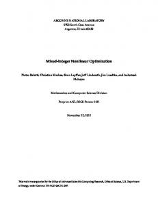
by taking the initial leader variables as parameters, each follower programming uses the lower-level GA to obtain the best solution in the last generation. Note that the best solution in the last generation provided by the lower-level GA is a good approximation for the optimal solution, which meets the lower-level constraints. Then the lower-level approximation solutions are brought back to the upper-level GA to solve the leader program. In the upper-level GA, the solutions should be verified whether they satisfy the leader’s constraints. The second assumption is that the algorithm has convergence. As the proposed BLGA meets the first condition, it can obtain the optimal solution only if it has convergence, which is an important measurement of computing capacity. Convergence of a GA means that the last cycle of a finite series of cycles can yield the optimal solution. This assumption ensures that, after comparing feasible solutions, the optimal solution can be found. An algorithm is only effective and feasible when it satisfies this condition. Currently, many GAs have been designed to solve special types of problems that have convergence [28–30]. Markov chains are often used to evaluate convergence. If a GA whose mutation rate is fixed and greater than 0 takes an elitist strategy and the binary code strategy, it has convergence that cannot be influenced by the initial population. Using the elitist strategy allows the best chromosome to be removed from operations in order to avoid disappearing in the operations. Moreover, many factors influence convergence, such as the maximal number of generations, crossover rate, mutation rate, and crossover and mutation methods. According to the above assumptions, even though the best solution provided by the BLGA does not guarantee to be the optimal solution, it may be a good approximation for the global optimal solution in reasonable time. We can calculate the problem several times, using different seeds, to find the closest approximation solutions. Numerical examples are given in Section 3.4 to verify the algorithm. 3.2. Design Process of BLGA. On the basis of the above assumptions, this study proposes a BLGA to solve MINLBLP with one or multiple independent followers that can improve efficiency in generating solutions. The essential process is as follows. First, leader decision variables are initialized according to their bound constraints. Second, each lower-level GA takes leader decision variables 𝑋 = {𝑥1 , 𝑥2 , . . . , 𝑥𝑖 , . . . , 𝑥𝑚 } as parameters to solve the 𝑖th follower problem to determine the best solution 𝑌𝑖∗ (𝑋) and the value of 𝑓𝑖∗ (𝑋, 𝑌𝑖∗ (𝑋)), where 𝑖 = 1, . . . , 𝑛. Third, the best solution 𝑌𝑖∗ (𝑋) for each follower and the leader decision variables 𝑋 is returned to the leader problem to determine if they satisfy other leader constraints. Their fitness values are then evaluated. Fourth, selection, crossover, and mutation operations are performed for these leader decision variables. Fifth, this cycle continues until maximal iterations are reached. The best optimal solutions 𝑋∗ and 𝑌1∗ , . . . , 𝑌𝑛∗ are then recorded. However, there is no guarantee that the optimal solutions will be the best solution for MINLBLP with one or multiple independent followers because the GA can only ensure that solutions belong to the constraint region rather than the

4


Start

Compare each optimal solutions and record the best one

Return

Reach? (i) Maximal number of runs(k)

Yes

No Initial leader population {X} (i) Population size {Nf } (ii) Leader bound constrains Initial follower population {Y(X)} (i) Parameters: leader chromosomes {X}

Verify? (i) Leader constrains

Yes

Exist? (i) Follower best chromosome Y∗ (X)

Yes

No Fitness evaluation (i) Evaluation function {Fmax − F(X, Y)}

Y∗ (X)

Fitness evaluation (i) Dynamic penalty function

No

Set fitness value = 0

Reach? (i) Maximal number of generations

Record follower best chromosome Y∗ (X)

Yes

Reach? (i) Maximal number of generations No

Yes

Sequence chromosomes (i) Cumulative probability

No Sequence chromosomes (i) Cumulative probability

Select good chromosomes for reproduction (i) Roulette wheel selection

Select good chromosomes for reproduction (i) Roulette wheel selection

Crossover (i) Crossover rate (ii) Uniform crossover

Crossover (i) Crossover rate (ii) Uniform crossover

Record leader best chromosome X∗ and follower best chromosome Y∗ (X∗ )

Mutation (i) Mutation rate (ii) Uniform mutation

Mutation (i) Mutation rate (ii) Uniform mutation

Figure 1: Process of the proposed BLGA.

inducible region. It is necessary to run this process several times to obtain several optimal solutions. These optimal solutions are then compared to determine the best solution. The process of the proposed BLGA is shown in Figure 1.

number. To determine if the termination condition has been satisfied, the maximal number of runs 𝑘 must be input. If this condition is satisfied, each optimal solution is compared to determine the best solution. If the termination condition is not satisfied, the process proceeds to Step 2.

3.3. BLGA Procedure. The procedure of the proposed BLGA is as follows.

Step 2 (initialize the leader population with leader population size 𝑁𝐹 ). According to their bound constraints, the leader population is initialized and these variables are encoded. Two strategies are used for the encoding of variables. The proposed method uses the binary code strategy, which uses

Step 1 (verify if the process is terminated). The termination condition is that the number of runs has reached the maximal


5

binary vectors as chromosomes, to represent the values of continuous variables with unequal lengths. The variable encoding length 𝑙 is expressed as follows: 𝑙 = [log2 (

𝑢max − 𝑢min )] + 1, 𝛿

(8)

where 𝑢max and 𝑢min represent the upper and lower bounds of the variables, respectively, and 𝛿 is precision. The proposed method also uses the real code strategy for encoding, which uses ordered arrays to represent discrete variable values. Step 3 (run lower-level GAs). Each follower programming takes the initial leader population 𝑋 = {𝑥1 , 𝑥2 , . . . , 𝑥𝑖 , . . . , 𝑥𝑚 } as a parameter. Note that the processes for each lower-level GA are the same. First, the follower population size 𝑁𝑓 is input, and the follower population is initialized according to their bound constraints. The two strategies described in Step 2 are used to encode the population. Second, verify that the follower chromosomes satisfy the follower constraints. If the follower chromosome does not satisfy the requirement, set the fitness values of it to zero. The others are evaluating the fitness value based on the follower objective function. Third, the maximal number of generations is input to verify whether the current number of generations is equivalent to the maximal number. If the current generation reaches the maximal number, the best follower chromosome 𝑌𝑖∗ (𝑋), 𝑖 = 1, . . . , 𝑛, is recorded and the solution’s feasibility is verified. If the solution meets the lower-level constraints, it is returned to the leader program or else null is returned. If the current population does not reach the maximal number, selection, crossover, and mutation operations are performed and the process continues. Step 4 (calculate the leader fitness evaluation). The leader programming takes the best chromosome of each follower 𝑌𝑖∗ (𝑋), 𝑖 = 1, . . . , 𝑛, as a parameter. Then, verify if 𝑌𝑖∗ (𝑋), 𝑖 = 1, . . . , 𝑛, are null values. If at least one is null, the fitness value is set to zero. If no null values are found, (𝑋∗ , 𝑌1∗ (𝑋), . . . , 𝑌𝑛∗ (𝑋)) are taken into the leader constraints. If it satisfies the constraints, the objective function 𝐹(𝑋∗ , 𝑌1∗ , . . . , 𝑌𝑛∗ ) is calculated and all 𝐹(𝑋∗ , 𝑌1∗ , . . . , 𝑌𝑛∗ ) are sorted in descending order to obtain the largest value, that is, 𝐹max . The current 𝐹max is compared with the previous 𝐹max , and the larger value is recorded as the new 𝐹max . The fitness function 𝐹max − 𝐹(𝑋∗ , 𝑌1∗ , . . . , 𝑌𝑛∗ ), which can ensure nonnegative fitness values, is used to evaluate the individuals and record their fitness values. If the constraints are not satisfied, the fitness value is set to zero. Step 5 (verify if the cycle is terminated). The termination condition is that the number of generations has reached the maximal number. If the maximal number is reached, the chromosome with the greatest fitness value is considered the best solution. The best leader chromosome 𝑋∗ and each best follower chromosome 𝑌𝑖∗ (𝑋), 𝑖 = 1, . . . , 𝑛, for each generation are recorded and the process returns to Step 1. If the maximal number has not been reached, the process continues to Step 6. Note that inputting a correct maximal number of generations is very important to an algorithm’s

convergence. If the number is too small, the algorithm may not find the best solution after termination of the cycle. In contrast, if the number is too large, efficiency may be reduced. A careful and deliberate choice is required. Step 6 (selection operation). The roulette wheel selection method is used to select 𝑁𝐹 −1 good chromosomes as parents for the crossover operation. Simultaneously, another good chromosome is selected as the best chromosome within the current population according to the elitist strategy. Step 7 (crossover operation). Input the crossover rate 𝑝𝑐 . Each of the parents selected in Step 6 is picked randomly, and each pair uses a uniform crossover method to undergo crossover with the given probability. Note that the new population includes these new chromosomes. Step 8 (mutation operation). The proposed method uses two mutation methods. For continuous variables that use the binary code strategy for encoding, the mutation rate 𝑝𝑚 is input and the uniform mutation method with the given probability is used. For discrete variables that use the real code strategy, new chromosomes are formulated as follows: 𝑥𝑖∧ = [(𝑥𝑖 − lb𝑖 + 1) mod (ub𝑖 − lb𝑖 )] + lb𝑖 ,

(9)

where 𝑥𝑖 and 𝑥𝑖∧ are the individuals before and after mutating, respectively, and lb𝑖 and ub𝑖 are the lower and upper bounds of the integer variables, respectively. After completion of Step 8, the process returns to Step 3. 3.4. Numerical Examples. The proposed BLGA for solving MINLBLP with one or multiple independent followers is realized using MATLAB. To verify the effectiveness and robustness of the proposed BLGA, we give numerical examples obtained with a personal computer with the following parameters: population size is 50; maximal number of generations is 200; precision of binary code is 0.01; crossover rate is 0.8; mutation rate is 0.01; number of experiments is fifteen. The results were compared with the exact solutions obtained from traditional methods for solving MINLBLP to test the quality of the computed solution. The best, worst, average, and median results and standard deviation value are presented. Example 1 (leader and follower decision variables are discrete). min 𝐹 (𝑋, 𝑌) = −𝑥1 2 − 3𝑥2 − 4𝑦1 2 + 𝑦2 2 𝑋

𝑥1 2 + 2𝑥2 2 − 4 ≤ 0 𝑥1 + 𝑥2 − 𝑦1 − 𝑦2 ≤ 0 𝑥1 ∈ {0, 1, 2} 𝑥2 ∈ {0, 1, 2}

6

Mathematical Problems in Engineering Table 1: Results of Example 1. ∗

∗

∗

∗

Table 2: Results of Example 2. ∗

∗

∗

∗

𝐹 (𝑋 , 𝑌 ) 𝑋 𝑓 (𝑋 , 𝑌 ) 𝑌 Best 0 (1, 1) −8 (0, 2) Worst 0 (2, 0) −2 (0, 2) Average 0 — −5.60 — Median 0 — −8 — Standard deviation value 0 — 3.04 — Enumeration method 0 (1, 1) −8 (0, 2)

𝐹∗ (𝑥∗ , 𝑦∗ ) 𝑥∗ 𝑓∗ (𝑥∗ , 𝑦∗ ) 𝑦∗ Best 12.0030 6.0000 −2.0010 2.0010 Worst 12.1596 5.9217 −2.0793 2.0793 Average 12.0134 — −2.0010 — Median 12.0030 — −2.0070 — Standard deviation value 0.0404 — 0.0217 — Graphic method 12.0000 6 −2.0000 2.0000

min 𝐹 (𝑋, 𝑌) = 2𝑥1 2 + 𝑦1 2 − 5𝑦2 𝑌

− 2𝑦1 + 𝑦2 ≤ 3 + 𝑥1 2 − 2𝑥1 + 𝑥2 2 𝑦1 ∈ {0, 1, 2} 𝑦2 ∈ {0, 1, 2} . (10) Example 1 is a simple integer nonlinear BLP problem that can be solved using the enumeration method. The best, worst, average, and median results and standard deviation value are shown in Table 1. Table 1 shows the results of Example 1. The standard deviation value of 𝐹∗ (𝑋∗ , 𝑌∗ ) is zero, which means that each run of this BLGA in this test finds the same upper objective function value. However, the standard deviation of 𝑓∗ (𝑋∗ , 𝑌∗ ) is 3.04, which means that there exists more than one optimal solution found by the proposed BLGA in this example. From the result of each run, we find that the solutions 𝑋 = (2, 0) and 𝑋 = (1, 1) are the optimal solutions. However, even though both of these solutions have the same upper optimal solution, their lower optimal solutions are different. When the upper-level solution is 𝑋 = (2, 0), the lower-level result is −2. When the upper-level solution is 𝑋 = (1, 1), the lower-level result is −8. The upper solution 𝑋 = (1, 1) provides a better value for the lower-level objective function. Therefore, the best solution for this test is 𝑋 = (1, 1) and 𝑌 = (0, 2). The iterative process is shown in Figure 2. As seen in Figure 2(a), the maximal number of generations does not need to be 200 because the optimal solution has been determined in the first generation. Figure 2(b) shows the BLGA evolution processes for the upper-level and lower-level optimizations. Example 2 (continuous leader and follower decision variables). 𝐹 (𝑥, 𝑦) = 𝑥 + 3𝑦 min 𝑥 𝑦−𝑥≤0 1≤𝑥≤6 min 𝐹 (𝑥, 𝑦) = −𝑦 𝑦 𝑥+𝑦≤8 − 𝑥 − 4𝑦 ≤ −8 𝑥 + 2𝑦 ≤ 13.

(11)

Example 2 is simple continuous BLP that can be solved by the graphic method. The best, worst, average, and median results and standard deviation value are shown in Table 2. As can be seen, the difference between the values of upper-level objective functions of the best result calculated by the proposed BLGA and the exact method is 0.0030, which is a negligible difference. This demonstrates the effectiveness of the proposed BLGA. In these 15 independent runs, except the worst result, the other results are the same. The iterative process of the best result is shown in Figure 3(a). As can be seen, the maximal number of generations does not need to be 200 because the optimal solution has been determined in the fifth generation. Figure 3(b) shows the BLGA evolution processes for the upper-level and lower-level optimizations. Example 3 (leader decision variables are discrete and follower decision variables are continuous).

min 𝐹 (𝑋, 𝑌) = − 𝑋

(𝑥1 + 𝑦1 ) (𝑥2 + 𝑦2 ) 1 + 𝑥1 𝑦1 + 𝑥2 𝑦2

𝑥1 2 + 𝑥2 2 ≤ 100 𝑥1 2 − 𝑥2 2 ≤ 𝑦1 2 − 𝑦2 2 𝑥1 ∈ {0, 1, 2, 3, 4, 5, 6, 7, 8, 9, 10} 𝑥2 ∈ {0, 1, 2, 3, 4, 5, 6, 7, 8, 9, 10} min 𝐹 (𝑋, 𝑌) = 𝑌

(12)

(𝑥1 + 𝑦1 ) (𝑥2 + 𝑦2 ) 1 + 𝑥1 𝑦1 + 𝑥2 𝑦2

0 ≤ 𝑦1 ≤ 𝑥1 0 ≤ 𝑦2 ≤ 𝑥2 . The results calculated by the proposed BLGA and the exact method are shown in Table 3. Table 3 shows the best and the worst results among these 15 runs, whose objective function values are the same as that calculated by the exact method, even though the solutions are different. The standard deviation value is near zero, which means that each independent run draws the similar objective function values. Figure 4(a) shows the iterative process of a best run, and the evolution processes for the upper-level and lower-level GAs are shown in Figure 4(b).


7

3

−7

0.5

Function value

2 1.5 1 0.5 0

−7.5

0

−8

−0.5

−1

−8.5

Function value of lower level

Function value of upper level

2.5

−0.5 −1

0

50

100 150 Number of generations

−1.5

200

0

The best objective function value of each generation The average objective function value of each generation

50

−9 200


The best objective function of the upper-level model The best objective function of the lower-level model

(a)

(b)

−1.6

13

15.5

−1.7

12.8

15

−1.8

12.6

14.5 14 13.5 13 12.5 12 11.5

0

50


200

12.4

−1.9

12.2

−2

12

−2.1

11.8

−2.2

11.6

−2.3

11.4

−2.4

11.2

−2.5

0


50



16


Function value

Figure 2: Iterative process of Example 1.

11 200

The best objective function of the lower-level model The best objective function of the upper-level model

(a)

(b)



Best Worst Average Median Standard deviation value Exact method

∗

∗

𝐹 (𝑋 , 𝑌 ) −1.9600 −1.9600 −1.9600 −1.9600 6.8951 × 10−16 −1.9600

𝑋∗ (7, 7) (7, 7) — — — (7, 7)

𝑓∗ (𝑋∗ , 𝑌∗ ) 1.9600 1.9600 1.9600 1.9600 6.8951 × 10−16 1.9600

𝑌∗ (7.0000, 0.0008) (0.0009, 7.0000) — — — (7.0000, 0.0000)

8

Mathematical Problems in Engineering 0

2

−1.6

1.9

−1.7

1.8

−1.8

1.7

−1.9


−0.4 Function value

−0.6 −0.8 −1 −1.2 −1.4 −1.6


−0.2

−1.8 −2

0

50

200



1.6

0

50


−2 200


(a)

(b)


Example 5 (MINLBLP with multiple independent followers).


∗

∗

∗

∗

∗

∗

𝐹 (𝑋 , 𝑌 ) 𝑥 𝑓 (𝑥 , 𝑦 ) Best 1.0000 1.0039 1.5319 × 10−5 Worst 1.0333 1.0011 1.1000 × 10−3 Average 1.0045 — 1.8139 × 10−4 Median 1.0000 — 1.5319 × 10−5 Standard deviation value 0.1171 — 0.0004 Exact method 1.0000 1.0000 0.0000

∗

𝑦 1 1 — — — 1

𝐹 (𝑥, 𝑌1 , 𝑌2 ) min 𝑥 = (𝑦11 + 𝑦21 − 200) (𝑦11 + 𝑦21 ) + (𝑦12 + 𝑦22 − 160) (𝑦12 + 𝑦22 ) 𝑥1 + 𝑥2 + 𝑥3 + 𝑥4 ≤ 40 𝑦11 + 𝑦22 ≤ 𝑥3 1 ≤ 𝑥1 ≤ 10

Example 4 (leader decision variables are continuous and follower decision variables are discrete). 𝐹 (𝑥, 𝑦) = (𝑥 − 1)2 + (𝑦 − 2) min 𝑥

1 ≤ 𝑥3 ≤ 15

2

1 ≤ 𝑥4 ≤ 20

𝑦−𝑥≤0

2

2

min 𝑓 (𝑥, 𝑌1 ) = (𝑦11 − 4) + (𝑦12 − 4) 𝑌1

1≤𝑥≤3 𝐹 (𝑥, 𝑦) = (𝑥 + 𝑦 − 2) min 𝑦

1 ≤ 𝑥2 ≤ 5

2

0.4𝑦11 + 0.7𝑦12 ≤ 𝑥1

(13)

0.6𝑦11 + 0.3𝑦12 ≤ 𝑥2

𝑥+𝑦≤5

0 ≤ 𝑦11 ≤ 20

𝑦 ∈ {0, 1, 2, 3} .

𝑦12 ∈ {0, 1, 2, . . . , 20} 2

The results are shown in Table 4. In these 15 runs, there are 6 times in which the proposed BLGAs draw the different solutions with the best result. However, these differences are so small that can be negligible. Moreover, the best result is rather similar to the exact solution, which demonstrates the effectiveness of the proposed BLGA. The iterative process is shown in Figure 5(a), and the BLGA evolution processes for the upper-level and lower-level optimizations are shown in Figure 5(b).

(14)

min 𝑓 (𝑥, 𝑌2 ) = (𝑦21 − 35) + (𝑦22 − 2) 𝑌2

0.4𝑦21 + 0.7𝑦22 ≤ 𝑥3 0.6𝑦21 + 0.3𝑦22 ≤ 𝑥4 0 ≤ 𝑦21 ≤ 40 𝑦22 ∈ {0, 1, 2, . . . , 40} . The results are shown in Table 5.

2


9 Table 5: Results of Example 5.

∗

Best Worst Average Median Standard deviation value Exact method

𝐹 −6598.6 −6512.8 −6568.81 6572.40 22.0338 −6600

𝑓1 ∗ 16.5284 54.8902 25.0162 9.8871 15.1987 11.9241

𝑋∗ (7.61, 4.66, 11.09, 16.64) (4.82, 2.90, 12.80, 19.38) — — — (7.91, 4.37, 11.09, 16.63)

𝑌1 ∗ (3.27, 9) (1.57, 6) — — — (2.29, 10)

𝑓2 ∗ 56.8328 12.94 52.3811 72.1481 22.4542 64.6841

1.5


Function value

5 4 3 2

2

1

1.5

0.5 1

0

0.5

−0.5

1

0

50


200


−1

0

50



2.5

6

0

𝑌2 ∗ (27.73, 0) (32.01, 0) — — — (27.21, 0)

0 200


(a)

(b)


Table 5 shows the basic information about these 15 independent runs. Note that the differences between the best objective function values calculated by the proposed BLGA and the exact method are negligible. The iterative process is shown in Figure 6(a), and the BLGA evolution processes for the upper-level and lower-level optimizations are shown in Figure 6(b). 3.5. Algorithm Evaluation. Based on the characteristic of MINLBLP with one or multiple independent followers in product family design (PFD), we have proposed a BLGA to solved this problem. We use five numerical examples to demonstrate the effectiveness and robustness of the proposed BLGA. We summarize the advantages of the proposed BLGA as follows. First, MINLBLP with one or multiple independent followers has generality, which can illustrate many practical management and engineering problems, such as PFD. Many studies have examined using GAs to solve special BLP problems. Some algorithms require that leader constraints include no follower decision variables, which cannot solve the target MINLBLP problems. In addition, some algorithms require only continuous decision variables, which limit practical application. In theory, the proposed BLGA has no limitations on constraints and variables.

Second, the optimal solutions calculated by the proposed algorithm belong to the constraint region. Note that to ensure the feasibility of the optimal solutions, we have made the following assumptions prior to designing the proposed BLGA. In the BLGA, the fitness values of individuals that do not satisfy constraints are set to zero to avoid being selected as parents. This ensures that the optimal solutions satisfy all constrains, which belong to the constraint region. Third, the proposed BLGA has good effectiveness and strong robustness, which has been demonstrated through the five numerical examples. Note that we use the binary code strategy to encode so that we can set the precision according to practical requirements. This strategy suits the mechanism of GAs, which can search for optimal solutions carefully.

4. Case Study 4.1. Problem Description. A case study of a simplified reducer family design is shown to demonstrate the proposed BLGA. A single-stage gear reducer includes three types of customized reducers, whose transmission ratios are 2, 3, and 4, respectively. To reduce cost and produce the three reducers simultaneously, we design platform parts and different customization parts, respectively. In this case, platform parts include a shell,

10

Mathematical Problems in Engineering −2500

150

−5500

100

−6000

50

−6500

Function value

−3500 −4000 −4500 −5000 −5500 −6000 −6500 −7000

0

50


200


0

0

50




−3000

−7000 200

The best objective function of the first lower-level model The best objective function of the second lower-level model The best objective function of the upper-level model

(a)

(b)


a high-speed shaft, and a low-speed shaft, whose critical parameters are taken as the platform variables. The different customization parts include the high-speed gear and the low-speed gear, whose critical parameters are taken as the customization variables. The critical parameter of platform parts is shell size, which is described by the center distance and diameter of high-speed shaft 𝑑𝐻. The center distance is proportional to the total number of gears when the module is determined; thus, we take the total number of gears 𝑧𝑠 as a platform variable. To optimize customization parts, we must optimize the selection of materials of gears 𝑦𝑖𝑗 (a 0-1 variable) and the number of teeth of high-speed gear 𝑧𝐻𝑖 (𝑖 = 1, 2, 3; the total number of gears is the sum of the number of lowspeed gear and high-speed gear teeth). Here, 𝑦𝑖𝑗 = 1 indicates that the 𝑖th reducer uses the jth material. In the design process of the reducer family, we cannot consider platform optimization and customization optimization simultaneously. The platform designer who optimizes the platform aims to leverage enterprise profitability, which includes maximizing the performance of all reducers and minimizing total cost. The customization designers design customization variables to maximize the performance of each reducer. Note that these designers have different goals and decision variables; however, their decisions affect each other. This is a joint optimization problem. Compared with the customization designers, platform designers act as leaders because the platform is the basis of a product family, which is more important. The customization designers act as followers. Consequently, this case can be considered a Stackelberg game-based decision-making problem. 4.2. Model Development. In this reducer family design problem, the leader is the platform design, whose decision variables are the total number of gears 𝑧𝑠 and the diameter of high-speed shaft 𝑑𝐻. The objective is to maximize the

performance of all reducers and minimize total cost. The constraints are the ranges of the decision variables. In this problem, the performance of the reducer family is the sum of the performance of each reducer, which is influenced by bending resistance and abrasion resistance. We use the bending fatigue stress of high-speed gear 𝜎𝐹𝐻𝑖 to define the bending resistance of the 𝑖th reducer because bending resistance affects the bending and fracture of a gear and, compared with a low-speed gear, the high-speed gear is easier to break. Because it is influenced by contact fatigue stress, the abrasion resistance is defined by the contact fatigue stress 𝜎𝐻𝑖 . In this simplified case, we describe the evolution of fatigue stress of the 𝑖th reducer by the product of two types of fatigue stress. The evolution of fatigue stress of the reducer family is ∑ 𝜎𝐻𝑖 𝜎𝐹𝐻𝑖 . This has an inverse relationship with the performance of the reducer; thus, the goal of maximizing the performance of all reducers can be replaced by minimizing the evolution of fatigue stress of the reducer family. Here, the total cost is the sum of the costs of each reducer, which is influenced by manufacturing materials. Assume that different types of reducers that use the same type of material have the same production cost. The customization designer can select the manufacturing materials from metals A, B, and C. The production costs 𝐶𝑗 (𝑗 = 1, 2, 3) are 50, 70, and 100, respectively. We define 𝑦𝑖𝑗 as 0-1 variables that show whether the 𝑖th reducer uses the jth material. The production cost of the 𝑖th reducer is ∑ 𝐶𝑗 𝑦𝑖𝑗 , and the production cost of the reducer family is ∑ ∑ 𝐶𝑗 𝑦𝑖𝑗 . We can describe the leader’s objective of the upper-level model as minimizing the product between the evolution of fatigue stress and the total cost, which is given as follows: min

3

3 3

𝑖=1

𝑖=1 𝑗=1

∑𝜎𝐻𝑖 𝜎𝐹𝐻𝑖 ∑ ∑𝐶𝑗 𝑦𝑖𝑗 .

(15)


11 Table 6: Material coefficients of metals. Metal A (𝑗 = 1) 200 MPa0.5

Metal B (𝑗 = 2) 190 MPa0.5

Metal C (𝑗 = 3) 180 MPa0.5

Contact fatigue stress [𝜎]𝐻𝑗

300 MPa

400 MPa

500 MPa

Bending fatigue stress [𝜎]𝐹𝐻𝑗

100 MPa

200 MPa

300 MPa

Elastic coefficient 𝑍𝐸𝑗

The lower-level models attempt to optimize the three types of reducers. For the 𝑖th reducer, the decision variables are the diameter of low-speed shaft 𝑑𝐿 𝑖 , the number of teeth of high-speed gear 𝑧𝐻𝑖 , and the materials selection variable 𝑦𝑖𝑗 (𝑖, 𝑗 = 1, 2, 3). The objectives of the lower-level models are to minimize the cost of reducer 𝐶𝑗 𝑦𝑖𝑗 . The constraints are the restrictions of fatigue stress, dimensions, ranges of indicators, ranges of variables, and material selections. The constraints of fatigue stress are that bending fatigue stress and the contact fatigue stress are less than allowable stress, respectively, which are given as follows: 3

𝜎𝐻𝑖 = 𝑍𝐻 ∑𝑍𝐸𝑗 𝑦𝑖𝑗 √ 𝑗=1

2𝐾𝑇𝐻𝑖

𝑏𝑖 𝑚2 𝑧𝐻𝑖 2

⋅

𝑢𝑖󸀠 + 1 𝑢𝑖󸀠

3

≤ ∑ [𝜎𝐻𝑖 ] 𝑦𝑖𝑗 ,

(16)

𝑗=1

𝜎𝐹𝐻𝑖 =

2𝐾𝑇𝐻𝑖 𝑌𝐹𝑆𝐻𝑖 𝑏𝑖 𝑧𝐻𝑖 𝑚2

3

Variables and indicators Diameters of high-speed shaft 𝑑𝐻 Total number of gears 𝑧𝑆 Diameters of low-speed shaft 𝑑𝐿 𝑖 Number of teeth of high-speed gear 𝑧𝐻𝑖 Transmission ratio of reducer 1 𝑢1 Transmission ratio of reducer 2 𝑢2 Transmission ratio of reducer 3 𝑢3

𝑗=1

𝐷𝐻𝑖 = 𝑚𝑧𝐻𝑖 ≥ 𝑑𝐻𝑖 + 20, 𝐷𝐿 𝑖 = 𝑚𝑧𝐿 𝑖 ≥ 𝑑𝐿 𝑖 + 20.

(17)

𝑧𝑆 − 𝑧𝐻𝑖 𝑧𝐻𝑖

≤ 𝑢𝑖𝐻.

𝑑𝐻 ,𝑧𝑆

s.t.

3

3 3

𝑖=1

𝑖=1 𝑗=1

∑𝜎𝐻𝑖 𝜎𝐹𝐻𝑖 ∑∑ 𝐶𝑗 𝑦𝑖𝑗 𝐿 𝑈 𝑑𝐻 ≤ 𝑑𝐻 ≤ 𝑑𝐻

𝑧𝑆𝐿 ≤ 𝑧𝑆 ≤ 𝑧𝑆𝑈 3

min

𝑑𝐿 𝑖 ,𝑧𝐻𝑖 ,𝑦𝑖𝑗

∑ 𝐶𝑗 𝑦𝑖𝑗

𝑗=1

3

s.t.

𝜎𝐻𝑖 = 𝑍𝐻 ∑ 𝑍𝐸𝑗 𝑦𝑖𝑗 √ 𝜎𝐹𝐻𝑖 =

2𝐾𝑇𝐻𝑖

𝑏𝑖 𝑚2 𝑧𝐻𝑖 2

2𝐾𝑇𝐻𝑖 𝑌𝐹𝑆𝐻𝑖 𝑏𝑖 𝑧𝐻𝑖 𝑚2

3

𝜎𝐻𝑖 ≤ ∑ [𝜎𝐻𝑖 ] 𝑦𝑖𝑗 𝑗=1

(18)

Each customization designer can only select a single material. This constraint is expressed as follows: 3

∑𝑦𝑖𝑗 = 1.

min

𝑗=1

Suppose the margin of error for the actual transmission ratio of the reducers is 10% above or below the nominal transmission ratio. The constraints of the indicator ranges include the ranges of the actual transmission ratio, which is expressed as follows:

Range 40–60 mm 140∼160 60–100 mm 25–60 1.8–2.2 2.7–3.3 3.6–4.4

the upper and lower bounds are represented by superscripts 𝑈 and 𝐿. According to our analysis, an MINLBLP model with multiple independent followers of the leader-follower joint optimization for the reducer family design can be expressed as follows:

≤ ∑ [𝜎𝐹𝐻𝑖 ] 𝑦𝑖𝑗 ,

where loading coefficient 𝐾 is 1.4, region coefficient 𝑍𝐻 is 2.5, tooth width 𝑏𝑖 is 80 mm, and the torque of the high-speed shaft is 1.27 × 105 N⋅mm. The different material coefficients of metal are given in Table 6. The dimension constraints dictate that the diameters of the reference circles of low-speed and high-speed gears are greater than 20 mm longer than the diameters of the low-speed shaft and high-speed shaft, respectively, which are given as follows:

𝑢𝑖𝐿 ≤ 𝑢𝑖 =

Table 7: Ranges of variables and indicators.

(19)

𝑗=1

In addition, there are also constraints for the ranges of variables. These constraints are given in Table 7. Note that

3

𝜎𝐹𝐻𝑖 ≤ ∑ [𝜎𝐹𝐻𝑖 ] 𝑦𝑖𝑗 𝑗=1

𝑚𝑧𝐻𝑖 ≥ 𝑑𝐻𝑖 + 20 𝑚 (𝑧𝑆 − 𝑧𝐻𝑖 ) ≥ 𝑑𝐿 𝑖 + 20 𝑢𝑖𝐿 ≤

𝑧𝑆 − 𝑧𝐻𝑖 𝑧𝐻𝑖

≤ 𝑢𝑖𝐻

⋅

𝑢𝑖󸀠 + 1 𝑢𝑖󸀠

12

Mathematical Problems in Engineering ×107 1.2

1.6

70

1.1

60

1

50

0.9

1.5 1.4 1.3 1.2 1.1 1

Overall evaluation of reducer family

80

1.7

Cost

0.9 0.8

0

50

100 150 200 Number of generations

250

40

300

0

50


Reducer A Reducer B

The best overall evaluation of each generation The average overall evaluation of each generation

250

0.8 300

Reducer C Reducer family

(a)

(b)

Evaluation of fatigue stress

×10 3

4

×107 1.2

1.1

2.5

1

2

0.9

1.5

1

0

50


250



×107 1.8

0.8 300

Reducer C Reducer family

Reducer A Reducer B (c)

Figure 7: Iterative process.

3

∑𝑦𝑖𝑗 = 1,

𝑗=1

𝑦𝑖𝑗 = 1 or 0

𝑑𝐿𝐿 𝑖 ≤ 𝑑𝐿 𝑖 ≤ 𝑑𝐿𝑈𝑖 𝐿 𝑈 𝑧𝐻 ≤ 𝑧𝐻𝑖 ≤ 𝑧𝐻 𝑖 𝑖

𝑖 = 1, 2, 3. (20) The material coefficient of metal and the ranges of variables and indicators are shown in Tables 6 and 7, respectively.

4.3. Solution and Analysis of Results. This model is an MINLBLP problem with three independent followers. We use the proposed BLGA to solve this problem with the following parameters: population size is 50; maximal number of generations is 300; precision of binary code is 0.01; and crossover rate is 0.8. Figure 7(a) shows that the best optimal solutions are found in the fiftieth generation. Figure 7(b) shows the evolution processes of the overall evaluation and cost. Figure 7(c) shows the overall evolution processes of the fatigue stress of the family and each reducer. The optimal results are given in Table 8, which shows the design of each reducer.

Reducer A Reducer B Reducer C

52.2627

159.6643

Platform variables Diameter of Total number of high-speed shaft gears 𝑧𝑆 𝑑𝐻 /mm

Table 8: Results. Customization variables Diameter of Number of teeth of Selections in metal low-speed shaft high-speed gear 𝑦𝑖𝑗 𝑑𝐿 𝑖 /mm 𝑧𝐻𝑖 77.4652 57.0171 A 64.0830 43.0684 A 79.6435 34.6496 B

50 50 79 8.7881 × 10

1.0337 × 105 1.7082 × 105 2.4275 × 105

Cost of reducer

Overall evaluation of reducer family 6

Evaluation of fatigue stress

Lower-level goal

Upper-level goal

Mathematical Problems in Engineering 13

14

5. Conclusion and Further Study MINLBLP can accurately model product family design, which has one or multiple nonlinear and nonconvex independent low-level models. Based on the characteristics of the model in product family optimization, the primary purpose of this study has been to propose a bilevel BLGA to solve product family optimization models. The proposed BLGA applies a GA to both the leader and followers and uses appropriate encoding strategies to handle continuous and discrete decision variables, which are common in product family optimization. The proposed BLGA overcomes many limitations of previously proposed GAs. For example, such GAs cannot solve a model in which leader constraints do not contain follower decision variables, which is common in product family optimization. The proposed BLGA overcomes this limitation. This paper models the joint optimization between product platform and product family designs by an MINLBLP approach in detail and presents a case study of a simplified reducer family design to demonstrate the feasibility and effectiveness of this model and BLGA. Currently, BLP is widely used in product family design optimization, which is a hot topic in engineering. GAs can solve BLP problems effectively. This paper only presents a specific application of a simplified reducer family design which describes the joint optimization between product platform design and product family design. In the future, we can do more research on other leader-follower relationships in the product family design problems and improve the BLGA efficiency by adjusting the encoding strategies and operation strategies.

Competing Interests The authors declare that there are no competing interests regarding the publication of this paper.

Acknowledgments This project is supported by the National Natural Science Foundation of China (nos. 71071104 and 71371132).

References [1] R. U. Nayak, W. Chen, and T. W. Simpson, “A variation-based method for product family design,” Engineering Optimization, vol. 34, no. 1, pp. 65–81, 2002. [2] S.-W. Hsiao, Y.-C. Ko, C.-H. Lo, and S.-H. Chen, “An ISM, DEI, and ANP based approach for product family development,” Advanced Engineering Informatics, vol. 27, no. 1, pp. 131–148, 2013. [3] B. Nepal, L. Monplaisir, and O. Famuyiwa, “Matching product architecture with supply chain design,” European Journal of Operational Research, vol. 216, no. 2, pp. 312–325, 2012. [4] X. Zhang and G. Q. Huang, “Game-theoretic approach to simultaneous configuration of platform products and supply chains with one manufacturing firm and multiple cooperative suppliers,” International Journal of Production Economics, vol. 124, no. 1, pp. 121–136, 2010.

Mathematical Problems in Engineering [5] G. Du, R. J. Jiao, and M. Chen, “Joint optimization of product family configuration and scaling design by Stackelberg game,” European Journal of Operational Research, vol. 232, no. 2, pp. 330–341, 2014. [6] Y. Kristianto, P. Helo, and R. J. Jiao, “Mass customization design of engineer-to-order products using Benders’ decomposition and bi-level stochastic programming,” Journal of Intelligent Manufacturing, vol. 24, no. 5, pp. 961–975, 2013. [7] G. Du, J. Yu, R. Y. Wu et al., “Leader-followers joint optimization of product family configuration and supply chain design,” International Journal of Knowledge, Innovation and Entrepreneurship, vol. 1, no. 1-2, pp. 6–23, 2013. [8] Y. Ji, R. J. Jiao, L. Chen, and C. Wu, “Green modular design for material efficiency: a leader-follower joint optimization model,” Journal of Cleaner Production, vol. 41, pp. 187–201, 2013. [9] R. J. Jiao and M. M. Tseng, “On equilibrium solutions to joint optimization problems in engineering design,” CIRP Annals— Manufacturing Technology, vol. 62, no. 1, pp. 155–158, 2013. [10] G. M. Wang, Z. P. Wan, and X. J. Wang, “Bibliography on bilevel programming,” Advances in Mathematics, vol. 36, no. 5, pp. 513– 529, 2007. [11] W. F. Bialas and M. H. Karwan, “Two-level linear programming,” Management Science, vol. 30, no. 8, pp. 1004–1020, 1984. [12] J. Fortuny-Amat and B. McCarl, “A representation and economic interpretation of a two-level programming problem,” The Journal of the Operational Research Society, vol. 32, no. 9, pp. 783–792, 1981. [13] G. Anandalingam and D. J. White, “A solution method for the linear static Stackelberg problem using penalty functions,” IEEE Transactions on Automatic Control, vol. 35, no. 10, pp. 1170–1173, 1990. [14] J. F. Bard, Practical Bilevel Optimization: Algorithms and Applications, Kluwer Academic Publishers, Amsterdam, The Netherlands, 1998. [15] S. Dempe, “Annotated bibliography on bilevel programming and mathematical programs with equilibrium constraints,” Optimization, vol. 52, no. 3, pp. 333–359, 2003. [16] B. Liu, “Stackelberg-Nash equilibrium for multilevel programming with multiple followers using genetic algorithms,” Computers & Mathematics with Applications, vol. 36, no. 7, pp. 79–89, 1998. [17] V. Oduguwa and R. Roy, “Bi-level optimisation using genetic algorithm,” in Proceedings of the 2002 IEEE International Conference on Artificial Intelligence Systems (ICAIS ’02), pp. 322–327, Divnomorskoe, Russia, 2002. [18] R. J. Kuo and Y. S. Han, “A hybrid of genetic algorithm and particle swarm optimization for solving bi-level linear programming problem—a case study on supply chain model,” Applied Mathematical Modelling, vol. 35, no. 8, pp. 3905–3917, 2011. [19] D.-Y. Lin, A. Unnikrishnan, and S. T. Waller, “A genetic algorithm for bi-level linear programming dynamic network design problem,” Transportation Letters, vol. 1, no. 4, pp. 281– 294, 2009. [20] Y. Fan and H. Li, “Genetic algorithm for solving linear bilevel programming with interval coefficients,” Journal of Computer Applications, vol. 34, no. 1, pp. 185–188, 2014. [21] H. Li, L. Zhang, and Y. Jiao, “Solution for integer linear bilevel programming problems using orthogonal genetic algorithm,” Journal of Systems Engineering and Electronics, vol. 25, no. 3, pp. 443–451, 2014.

Mathematical Problems in Engineering [22] H. Li, “A genetic algorithm using a finite search space for solving nonlinear/linear fractional bilevel programming problems,” Annals of Operations Research, vol. 235, pp. 543–558, 2015. [23] J. Lu, C. Shi, and G. Zhang, “On bilevel multi-follower decision making: general framework and solutions,” Information Sciences, vol. 176, no. 11, pp. 1607–1627, 2006. [24] H. I. Calvete and C. Gal´e, “Linear bilevel multi-follower programming with independent followers,” Journal of Global Optimization, vol. 39, no. 3, pp. 409–417, 2007. [25] J. S. Angelo and H. J. Barbosa, “Differential evolution to find Stackelberg-Nash equilibrium in bilevel problems with multiple followers,” in Proceedings of the 2015 IEEE Congress on Evolutionary Computation (CEC ’15), pp. 1675–1682, IEEE, Sendai, Japan, May 2015. [26] G. Du, R. J. Jiao, and M. Chen, “Joint optimization of product family configuration and scaling design by Stackelberg game,” European Journal of Operational Research, vol. 232, no. 2, pp. 330–341, 2014. [27] D. Wang, G. Du, R. J. Jiao, R. Wu, J. Yu, and D. Yang, “A Stackelberg game theoretic model for optimizing product family architecting with supply chain consideration,” International Journal of Production Economics, vol. 172, pp. 1–18, 2016. [28] M.-Y. Li, Z.-X. Cai, and G.-R. Sun, “An adaptive genetic algorithm with diversity-guided mutation and its global convergence property,” Journal of Central South University of Technology, vol. 11, no. 3, pp. 323–327, 2004. [29] B. Pavez-Lazo and J. Soto-Cartes, “A deterministic annular crossover genetic algorithm optimisation for the unit commitment problem,” Expert Systems with Applications, vol. 38, no. 6, pp. 6523–6529, 2011. [30] L.-Y. Zhuang, H.-B. Dong, J.-Q. Jiang, and C.-Y. Song, “A genetic algorithm using a mixed crossover strategy,” Lecture Notes in Computer Science, vol. 5263, no. 1, pp. 854–863, 2008.

15

Advances in

Operations Research Hindawi Publishing Corporation http://www.hindawi.com

Volume 2014

Advances in

Decision Sciences Hindawi Publishing Corporation http://www.hindawi.com

Volume 2014

Journal of

Applied Mathematics

Algebra

Hindawi Publishing Corporation http://www.hindawi.com


Volume 2014

Journal of

Probability and Statistics Volume 2014

The Scientific World Journal Hindawi Publishing Corporation http://www.hindawi.com


Volume 2014

International Journal of

Differential Equations Hindawi Publishing Corporation http://www.hindawi.com

Volume 2014

Volume 2014

Submit your manuscripts at http://www.hindawi.com International Journal of

Advances in

Combinatorics Hindawi Publishing Corporation http://www.hindawi.com

Mathematical Physics Hindawi Publishing Corporation http://www.hindawi.com

Volume 2014

Journal of

Complex Analysis Hindawi Publishing Corporation http://www.hindawi.com

Volume 2014

International Journal of Mathematics and Mathematical Sciences


Journal of

Mathematics Hindawi Publishing Corporation http://www.hindawi.com

Volume 2014


Volume 2014

Volume 2014


Volume 2014

Discrete Mathematics

Journal of

Volume 2014


Discrete Dynamics in Nature and Society

Journal of

Function Spaces Hindawi Publishing Corporation http://www.hindawi.com

Abstract and Applied Analysis

Volume 2014


Volume 2014


Volume 2014

International Journal of

Journal of

Stochastic Analysis

Optimization



Volume 2014

Volume 2014