Genetic Algorithm for Solving Site Layout Problem with Unequal-Size and Constrained Facilities P. P. Zouein, A.M.ASCE1; H. Harmanani2; and A. Hajar3 Abstract: This paper presents an investigation of the applicability of a genetic approach for solving the construction site layout problem. This problem involves coordinating the use of limited site space to accommodate temporary facilities so that transportation cost of materials is minimized. The layout problem considered in this paper is characterized by affinity weights used to model transportation costs between facilities and by geometric constraints that limit their relative positions on site. The proposed genetic algorithm generates an initial population of layouts through a sequence of mutation operations and evolves the layouts of this population through a sequence of genetic operations aiming at finding an optimal layout. The paper concludes with examples illustrating the strength and limitations of the proposed algorithm in the cases of 共1兲 loosely versus tightly constrained layouts with equal levels of interaction between facilities; 共2兲 loosely versus tightly packed layouts with variable levels of interactions between facilities; and 共3兲 loosely versus tightly constrained layouts. In most problems considered where the total-objects-to-site-area ratio did not exceed 60%, the algorithm returned close to optimal solutions in a reasonable time. DOI: 10.1061/共ASCE兲0887-3801共2002兲16:2共143兲 CE Database keywords: Algorithm; Construction sites; Workspace; Constraints.
Introduction and Background Construction site layout involves coordinating the use of limited site space to accommodate temporary facilities 共such as fabrication shops, trailers, materials, or equipment兲 so that they can function efficiently on site. The layout problem is generally defined as the problem of 共1兲 identifying the shape and size of the facilities to be laid out; 共2兲 identifying constraints between facilities; and 共3兲 determining the relative positions of these facilities that satisfy the constraints between them and allow them to function efficiently. There are different classes of layout problems that have been studied in the literature. The variations stem from the assumptions made on the shape and size of facilities and on the constraints between them. Facilities may have a defined shape and size or a loose shape, in which case they will assume the shape of the site to which they have been assigned 共for example, bulk construction material兲. The constraints can vary from simple nonoverlap constraints to other geometric constraints that describe orientation or distance constraints between facilities. In the layout problem addressed here, the shape and size of facilities are fixed. Facilities can have 2D geometric constraints on their relative positions 1
Assistant Professor, Dept. of Industrial Engineering, Lebanese American Univ., Byblos, Lebanon. E-mail:
[email protected] 2 Assistant Professor, Dept. of Computer Science, Lebanese American Univ., Byblos, Lebanon. 3 Graduate Research Assistant, Dept. of Computer Science, Lebanese American University, Byblos, Lebanon. Note. Discussion open until September 1, 2002. Separate discussions must be submitted for individual papers. To extend the closing date by one month, a written request must be filed with the ASCE Managing Editor. The manuscript for this paper was submitted for review and possible publication on April 16, 2001; approved on September 4, 2001. This paper is part of the Journal of Computing in Civil Engineering, Vol. 16, No. 2, April 1, 2002. ©ASCE, ISSN 0887-3801/2002/2143–151/$8.00⫹$.50 per page.
along with proximity weights describing the level of interaction or flow between them. The layout problem is an NP-complete combinatorial optimization problem, that is, optimal solutions can be computed only for small or greatly restricted problems 共Kusiak and Heragu 1987兲. Hence, layout planners often resort to using heuristics to reduce their search for acceptable solutions. These heuristics comprise strategic knowledge prescribing the order in which to select objects and to meet constraints, and have been modeled with various degrees of truthfulness, detail, and success in operations research and artificial intelligence applications for space planning 共Tommelein et al. 1991; Cheng 1992; Thabet 1992; Tommelein and Zouein 1993; Yeh 1995; Zouein 1995; Lin and Haas 1996; Feng et al. 1999; Zouein and Tommelein 1999兲. The application of genetic algorithms 共GAs兲 to solving layout problems is relatively recent. GAs work with a family of solutions, known as the ‘‘current population,’’ from which we obtain the ‘‘next generation’’ of solutions. When the algorithm is designed properly, we obtain progressively better solutions from one generation to the next. The main advantage of using GAs is in the fact that it only needs an objective function with no specific knowledge about the problem space. The challenge, however, remains in finding an appropriate problem representation that results in an efficient and successful implementation of the algorithm. GAs 共Goldberg 1989兲 have been applied to solving the facility layout problem 共FLP兲 in the area of production facilities 共Tanaka and Yoshimoto 1993; Tate and Smith 1993, 1995; Hamamoto et al. 1999兲 and to solving the ‘‘construction site-level facility layout’’ 共Li and Love 1998兲. In both applications, the layout problem was modeled as a location-allocation problem, which consists of allocating a set of predetermined facilities into a set of predetermined sites where the smallest site can accommodate the largest facility. GAs have not been used, however, to solve the site layout problem as defined in this paper. JOURNAL OF COMPUTING IN CIVIL ENGINEERING / APRIL 2002 / 143
This paper presents an evolutionary algorithm for optimally solving the site layout problem as characterized by affinity weights and 2D geometric constraints between facilities. The algorithm is tested on a variety of layout problems to illustrate its performance in the cases of 共1兲 loosely versus tightly constrained layouts with equal levels of interaction between facilities; 共2兲 loosely versus tightly packed layouts with variable levels of interaction between facilities; and 共3兲 loosely versus tightly constrained layouts. The paper concludes with a discussion of the capabilities and limitations of the proposed approach.
Geometrically Constrained Site Layout Problem The layout problem as modeled in this paper is characterized by rectangular layout objects with fixed dimensions representing the facilities to be positioned on site. Facilities can be positioned in one of two orientations only: a 0 or 90° orientation. In addition, facilities can have 2D constraints on their relative positions: namely, minimum and maximum distance, orientation, and nonoverlap constraints. Minimum and maximum distance constraints limit the distance between the facing sides of two facilities in the x- or y-direction to be greater than or less than a predefined value, respectively. Distance constraints can be used to model equipment reach or general clearance requirements. Orientation constraints limit a facility’s position to be to the north, south, east, or west of another reference facility. These constraints can be used to locate access roads or gates with respect to the main facility. Nonoverlap constraints are default constraints that restrict the positions of any two facilities from overlapping. The geometric constraints are considered hard constraints that should be satisfied for the layout to be feasible. The objective is to find a feasible arrangement for all layout objects within the site space that minimizes the sum of the weighted distances separating the layout objects 共Z兲: Z⫽⌺⌺ j⬍i 共 w i j ⫻d i j 兲
(1)
where w i j is the affinity weight between objects i and j that could be used to represent the flow or the unit transportation cost between i and j, and d i j is the rectilinear distance separating objects i and j. A feasible arrangement is obtained by finding positions for all layout objects that satisfy the 2D constraints between them.
Genetic Approach The basic notion of evolutionary computation is to mimic some principles of natural evolution in order to solve optimization problems of high complexity. A group of randomly initialized points of the search space 共individuals兲 is used to search the problem space. Each individual encodes all necessary problem parameters 共genes兲 as bit strings, vectors, or graphs. The population evolves following a parody of Darwinian principle of the survival of the fittest. Individuals are selected according to their quality, as measured by a fitness function, to produce offspring and to propagate their genetic material 共parts of the partial solution found so far兲 into the next generation. Each offspring undergoes a sequence of operators 共for example, mutation, inversion, and crossover兲 with a certain probability to provide diversity of the population, avoiding premature convergence to a single local optimum. The iterative process of selection and combination of ‘‘good’’ individuals should yield even better ones, until a solution is found or a certain stop criterion is met. 144 / JOURNAL OF COMPUTING IN CIVIL ENGINEERING / APRIL 2002
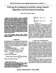
Fig. 1. 共a兲 N-E-S-W cut; 共b兲 E-S-W-N cut; 共c兲 S-W-N-E cut; 共d兲 W-N-E-S cut
Coding of Parameters A population is a collection of chromosomes where each chromosome represents a layout solution. Every chromosome is coded as a vector whose length is equal to the number of facilities that exist on site n. Each facility i is represented by the coordinates of its position on site: X i , Y i , by its dimensions: L i , W i ; and by a series of pointers pointing at the facilities that surround it in the four directions: north, south, east, and west. These pointers will be used to facilitate the check for overlap. The fitness function used is Z.
Genetic Operators A number of genetic operators is used to evolve an initial population to the optimal solution. These operators are slight variations of the traditional mutation, reproduction, and cross-over operators. The genetic operators used call for the Find-a-Set-ofPossible-Positions function 共simply termed here as Find-ASPP兲 that generates a set of feasible positions for an object in the neighborhood of a randomly selected location on site. This function takes as input a given location 共say, P兲 and returns a set of four rectangles or less that together describe feasible positions of the centerpoint of the object to be positioned by making vertical and horizontal cuts through the site, as shown in Fig. 1. Fig. 1 illustrates how Find-ASPP generates the four rectangles given some previously positioned facilities on the site 共represented by the gray-shaded rectangles兲 and a selected location P 共marked as x兲 for the object to be positioned 共shown outside the site space and labeled O-i兲. The first rectangle 关Fig. 1共a兲兴 is generated by making, first, a horizontal cut 共cut 1兲 through the edge of the closest object north of P, then a vertical cut 共cut 2兲 through the edge of the closest object east of P in the half space containing P and generated by the first cut. Cut 2 divides the half-space in two: the one containing P is retained to make the next cuts. A third horizontal cut 共cut 3兲 is made through the edge of the closest object to the south of P
in the space defined by the two previous cuts. Finally, a vertical cut 共cut 4兲 is made through the edge of the closest object to the west of P in the space containing P and defined by the previous three cuts. This last cut defines the fourth edge of the first rectangle generated by Find-ASPP 关see the cross-hatched rectangle in Fig. 1共a兲兴. The second rectangle 关shown as the cross-hatched rectangle in Fig 1共b兲兴 is generated similarly to the first, except that the cuts are done starting with the cut to the east and proceeding clockwise to finish with a cut to the north. The third and fourth rectangles 关Figs. 1共c-d兲, respectively兴 are generated similarly, starting with the south and west cuts, respectively, and moving clockwise to perform the remaining cuts. Finally, Find-ASPP reduces the length and width of each rectangle found by half the length and width of O-i, respectively, and returns the set of reduced rectangles that represent a feasible set of positions for O-i. Fig. 1共a兲 shows one such reduced rectangle in white with dotted edges inside the cross-hatched rectangle. Note that if the length and/or width of the object exceeds those of any of the rectangles found by Find-ASPP, then that rectangle is discarded from the set of rectangles returned by Find-ASPP. Note that Find-ASPP does not find the complete set of feasible positions of an object on site; rather, it finds a subset of those in the neighborhood of a suggested location. Also note that if the cuts were performed in an anticlockwise direction, the resulting rectangles returned by the function would be different from those shown in Fig. 1. If the order of the cuts is altered, the rectangles would be different as well. Enhancement of the Find-ASPP function can look at broadening the range of feasible positions that it returns by varying the order of the cuts and the direction followed. The genetic operators used are the following: 1.
2.
3.
4.
5. 6.
7.
Mutation selects a random location 共X, Y兲 and calls the FindASPP function to determine the range of feasible positions in the neighborhood of that location where the block can be inserted and not overlap with other blocks positioned on site, as shown in Fig. 1. If the block cannot be inserted—that is, Find-ASPP returns the null set—then the operation is aborted. Inversion flips a block’s position across a horizontal or vertical axis passing through the centroid of the site. This operator also uses the Find-ASPP function to determine if a range of feasible positions exists at the new position. If none exists, then the operation is aborted. Flip2Edge is an operator similar to inversion, with one difference: the axes pass through the centroid of a randomly selected reference block and not the site. Swap exchanges the positions of two randomly selected blocks in a chromosome. It is possible that either block may not fit in the place of the other block. If at least one block fits, then the other block is mutated, or else the operation is aborted. Rotation rotates a block 90° anticlockwise about its upperleft corner. Move moves a randomly selected block in a chromosome d units in the X- or Y-direction. The value of d is either Gaussian or unity, depending on the number of iterations in which the best solution did not change. Add-missing-blocks act on chromosomes that contain missing blocks—that is, blocks for which no feasible position was found in the initialization phase 共see next section for details兲. This may happen as a result of an inefficient use of
the site space. This operator attempts to find feasible positions for the missing blocks in a chromosome by applying a sequence of mutations. 8. Fix blocks fixes the positions of two blocks that have distance or orientation constraints between them. 9. Aging destroys chromosomes whose fitness value did not change after x iterations where x is set to 50 and could be changed to influence the rate of convergence. This operator is intended to age solutions that will not lead to the optimal one and allow young chromosomes to evolve into better solutions. Note that operators 1 through 7 call Find-ASPP to determine a Set of Possible Positions 共ASPP兲 for the centroid of the block operated on in the neighborhood of the new suggested location. If Find-ASPP returns the null set, then the operation calling it is aborted. If the new suggested location belongs to the set returned by Find-ASPP, and if all geometric constraints between the object under consideration and the previously positioned objects on site are satisfied at the new suggested location, then the object is inserted at that location. Otherwise, another location is selected at random from the set of positions returned by Find-ASPP. That new location is checked to see if it satisfies all geometric constraints on the object under consideration; if not, then another location is sampled at random from the ASPP. This process of sampling locations from the set of feasible positions returned by Find-ASPP is repeated up to n times where n is set arbitrarily to 20. If still no location is found to satisfy the geometric constraints, then the operation calling Find-ASPP is aborted.
Initialization Phase Chromosomes in the initial population are generated randomly by applying a sequence of mutation operations. First, blocks with user-defined fixed positions on site are added to a chromosome; these blocks cannot be moved by the above GA operations. Next, mutation is applied on the remaining blocks by selecting randomly a block at a time. If applying mutation on a given block results in an infeasible range for block insertion, then mutation is repeated on the same block up to 100 times to find a feasible position for that block. If after 100 trials no feasible position is found, this block is left out of the chromosome. Hence, this method may result in chromosomes representing partial layout solutions. The operator Add-Missing-Blocks will be responsible for completing such partial solutions in the evolutionary phase.
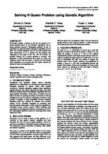
Evolutionary Phase Following the generation of the initial population, the genetic operators are applied to evolve the initial population into better ones as depicted in the flow chart of Fig. 2. Every operator has a probability associated with it. The product of the operator’s probability and the population size determines the maximum number of times this operator can be fired in one generation. Operator’s probabilities and values of other parameters were determined experimentally and are as shown in Table 1. Also experimentally, it was found that the pure survival of the fittest does not always work for this type of layout problems. Hence some ‘‘bad’’ chromosomes 共that is, chromosomes representing partial solutions or chromosome with high fitness value兲 were preserved in the next generation as this could in the long run help the algorithm converge to a global optimum. The following criteria were used in selecting chromosomes for reproduction: JOURNAL OF COMPUTING IN CIVIL ENGINEERING / APRIL 2002 / 145
Table 2. Input for Case 1 Problems
Problem 1 2 3 4
关Fig. 关Fig. 关Fig. 关Fig.
3共a兲兴 3共b兲兴 3共c兲兴 3共d兲兴
Number Dimensions W i j , ᭙i, of objects of object and ᭙ j 10 25 45 60
2⫻1 2⫻1 2⫻1 2⫻1
1 1 1 1
Total object-to-sitearea ratio 共OSAR兲 共%兲 10 23 40 54
Examples Application The proposed GA was run on different sets of problems to test the algorithm’s performance as the total object-to-site-area ratio 共OSAR兲 is varied in the following cases: equal size with equal weight objects, unequal size with unequal weight objects, unequal size with unequal weight objects, and 2D constraints between objects. In all these cases, the population size is set to 100 and the number of generations is limited to 400.
Case 1: Layout of Equal-Size with Equal-Weight Objects
Fig. 2. Flow chart of proposed genetic algorithm
1. 2.
3.
4.
Choose 5% from the best chromosomes; Randomly choose 10% from ‘‘bad’’ chromosomes with density fitness less than 60% or more that 150% of the best chromosome. The density fitness is the ratio between fitness value and number of blocks available in the chromosome. Note that a chromosome’s fitness value can exceed 100% if the chromosome represents a partial solution; Randomly choose 80% from those chromosomes with density fitness between 80 and 120% of the best chromosomes; and Choose randomly the remaining chromosomes.
Table 1. Operators and Probabilities Parameter
Value
Population size Probability of mutation Probability of move Probability of inverse
100 0.1 1 0.1
Parameter Probability of rotation probability of swap Probability of Flip2Edge Maximum age for aging
Value 0.2 0.1 0.2 50
146 / JOURNAL OF COMPUTING IN CIVIL ENGINEERING / APRIL 2002
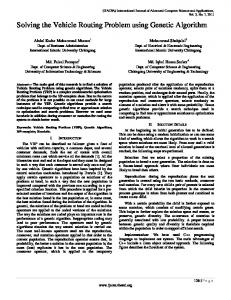
In this section, the GA is used to solve bin-packing-like problems where objects have the same dimensions and have equal weights between them. No geometric constraints were considered between objects for problems in this case. The four problems selected and shown here illustrate the GA’s performance in solving problems with different numbers of objects to be laid out 共10, 25, 45, and 60 objects兲 and thus different OSARs. Table 2 shows the input used with the four problems of Case 1. Fig. 3 shows, to the left, the best layout solution found by the GA and, to the right, the optimal solution or the best incumbent found for each of the four problems. Note that, for some problems, there exist alternative optimal layouts, only one such layout is shown in Fig. 3. Table 3 shows a comparison between the fitness value of the layouts generated by the GA along with the run-time of each problem and the optimal or ‘‘best’’ layouts found. The GA solutions found are on average within 5% of the optimal solution. This is considered a very good result, given the size of the problems solved. The GA was tested on a variety of other problems of the same class of problems shown here, that is, with equal size objects and equal weights between them. It returned solutions that are equally good for OSAR values up to 50%. The ‘‘goodness’’ of the GA solutions, however, deteriorates when the OSAR is raised above 60%.
Case 2: Layout of Unequal Size with Unequal Weight Objects In this section, the GA is used to solve layout problems with layout objects of different dimensions and having different weights between them 共that is, with different levels of interactions between them兲. No geometric constraints were considered for problems in this case as well. The four problems selected and shown here have the same OSAR as the four problems of Case 1. This choice is intentional to test how the GA’s performance varies when layout objects are not all equal. The inputs associated with the four problems are as shown in Table 4. Fig. 4 shows, on the left, the layout solutions returned by the GA, and on the right, the optimal or best incumbent solution for
OSAR less than 50% are on average within 6% from the optimal solution. The ‘‘goodness’’ of the solution drops suddenly for problems with OSAR greater than 50% as it is illustrated by the solution of problem 4 共Fig. 4共d兲; Table 5兲.
Case 3: Layout of Unequal Size with Unequal Weight and 2D Constraints between Objects
Fig. 3. 共Left兲 GA solution and 共right兲 optimal or best solution of 共a兲 Case 1 problem 1; 共b兲 Case 1 problem 2; 共c兲 Case 1 problem 3; 共d兲 Case 1 problem 4
each of the four problems described in Table 3. Table 5 shows a comparison between the fitness value of the layouts generated by the GA along with the run-time of each problem and the optimal or ‘‘best’’ layouts found. The GA solutions for problems with
Finally, this section treats the class of layout problems where objects are of different size and have variable weights between them and have geometric constraints on their relative positions in addition to the default nonoverlap constraints. Only two problems are presented in this section. These problems are intended to test the GA’s performance in solving problems with a relatively smaller number of layout objects, but with a larger variety of geometric constraints between them. The layout objects’ dimensions and proximity weights between them for both problems are given in Tables 6 and 7, respectively. Both problems have an OSAR value of approximately 50%. The first problem has in addition to the weights defined in Table 6, the following geometric constraints between objects: Object 6 is constrained to be to the north of object 7, and object 9 and object 10 should have a minimum distance of 5 units in the Y-direction between them. The GA solution to the above problem is shown in Fig. 5 共left兲 and has a fitness value of 1,325. Note that the gray-shaded rectangle represents object 4. The optimal solution for this problem has a fitness value of 1,262.5. There are alternative optimal layouts for this problem. Fig. 5 shows only one such optimal layout. The second problem considered has the same objects and relationships between them as the previous one. It has, however, two additional geometric constraints, namely, a maximum distance constraint of 8 units in the Y-direction between object 5 and object 7 and a minimum distance constraint of 5 units in the Y-direction between object 1 and object 10. The GA solution to this problem is shown in Fig. 6 共left兲 and has a fitness value of 1,350. The optimal solution to this problem is the same as for the previous problem and is shown in Figs. 5 and 6 共right兲. Table 8 summarizes the results of this last case. As can be seen, the proposed GA found solutions for problems with an OSAR value of 50% that are within 7% of the optimal solution. The GA’s performance drops when used on problems with higher OSAR values and a larger number of geometric constraints between objects.
Analysis of Results As can be seen from the results shown in Tables 3, 5, and 8 and summarized in Table 9, the GA found close to optimal solutions
Table 3. Comparison between GA Optimal or Best Incumbent Solution for Case 1 Problems Problem 1 2 3 4
关Fig. 关Fig. 关Fig. 关Fig.
3共a兲兴 3共b兲兴 3共c兲兴 3共d兲兴
OSAR 共%兲
GA solution fitness value
Time 共s兲
Optimal or best incumbent fitness value
Error 共%兲
10 23 40 54
135 1,438 6,226 12,145
144 406 1,336 1,851
131 1,407 5,852 12,389
3 2 6 2
JOURNAL OF COMPUTING IN CIVIL ENGINEERING / APRIL 2002 / 147
Table 4. Input for Case 2 Problems Problem 1 关Fig. 4共a兲兴
Objects
L⫻W
Number of objects
1
4⫻2
1
2, 3, 4, 5
2⫻2
4
Wij
OSAR 共%兲 10
5; ᭙i⫽2,...,5 ᭙ j⫽i⫹1⫽2,...,5 20; i⫽1 and j⫽2
2 关Fig. 4共b兲兴
1, 2, 3
4⫻2
3
10; ᭙i⫽1,...,3 ᭙ j⫽i⫹1⫽1,...,3
4, 5, 6, 7, 8, 9, 10
2⫻2
7
5; ᭙i⫽4,...,10 ᭙ j⫽i⫹1,...,10
23
20; i⫽1 and j⫽4 i⫽2 and j⫽5 3 关Fig. 4共c兲兴
1, 2, 3, 4, 5, 6, 7
4⫻2
7
10; ᭙i⫽1,...,7 ᭙ j⫽i⫹1,...,7
8, 9, 10, 11, 12, 13, 14, 15
2⫻2
8
5; ᭙i⫽8,...,15 ᭙ j⫽i⫹1,...,15
40
20; i⫽1 and j⫽8 i⫽2 and j⫽9 i⫽3 and i⫽10 4 关Fig. 4共d兲兴
1, 2, 3, 4, 5, 6, 7, 8, 9, 10
4⫻2
10
10; ᭙i⫽1,...,10 ᭙ j⫽i⫹1,...,10
11, 12, 13, 14, 15, 16, 17, 18, 19, 20
2⫻2
10
5; ᭙i⫽11,...,20 ᭙ j⫽i⫹1,...,20
54
10; i⫽1 and j⫽11 i⫽2 and j⫽12 i⫽3 and j⫽13
共on average within 6% of optimal兲 for the three classes of layout problems considered. In the first class of problems, the geometric constraints were reduced to the default nonoverlap constraints, and the interactions among objects were equated across all pairs of layout objects. The intent was to test the GA’s capability in solving bin-packing-like problems. The optimal solution for this class of problems results in tightly packed objects, as shown in Fig. 3. For the four problems considered, the proposed GA returned exceptionally good results, with less than 5% error on the largest problem 共with 60 objects and 60% OSAR兲. The algorithm converged to a solution in less than 250 generations for all problems solved in this case. In the second class of problems, the GA’s performance was equally good except for problems where the total-objects-to-sitearea ratio exceeded 50% 共as in the case of problem 4兲. In this class of problems, the restrictions on the size and weights between objects were relaxed. The geometric constraints, however, remained restricted to nonoverlap constraints only between objects. The writers suspect that this sudden drop in performance could be due to the fact that the levels of interactions between objects were made different between different pairs of objects, thus shifting the problem from a single packing problem, as in the first case of problems, to many packing problems within a problem. In the third class of problems, the GA was tested on a number of problems, two of which were presented in this section. In this class of problems, all restrictions were relaxed. Objects have dif148 / JOURNAL OF COMPUTING IN CIVIL ENGINEERING / APRIL 2002
ferent dimensions, and different levels of interactions and geometric constraints between them. Here too, the GA returned very good solutions 共within 7% of optimal solutions兲 for problems with less than 55% OSAR. The GA’s performance is noted to drop for tightly packed problems 共that is, problems with OSAR higher than 60%兲 or problems with a large number of geometric constraints between objects. Hence, the proposed GA could be used to solve different classes of layout problems and is expected to return ‘‘good solutions’’ 共within 7% of optimal solutions兲. However, from the problems considered in this paper and others not shown here, one can conclude that the GA performed better in loosely constrained problems with a small total-objects-to-site-area ratio 共55% or less兲 even when the number of blocks was high. This result is expected because of the very nature of GAs.
Conclusions This paper presented the results of a pioneering investigation on the application of genetic algorithms for solving the site layout problem, as characterized by rectangular facilities with proximity requirements between them and with geometric constraints that further restrict their relative positions. Key features of the proposed algorithm are that it uses a large number of different GA operators to vary positions of objects around the site. The GA operators are programmed so that the chance of finding a feasible
Fig. 4. 共Left兲 GA solution and 共right兲 optimal or best solution of 共a兲 Case 2 problem 1; 共b兲 Case 2 problem 2; 共c兲 Case 2 problem 3; 共d兲 Case 2 problem 4
JOURNAL OF COMPUTING IN CIVIL ENGINEERING / APRIL 2002 / 149
Table 5. Comparison between GA Solution and Optimal or Best Incumbent Solution for Case 2 Problems
Problem 1 2 3 4
关Fig. 关Fig. 关Fig. 关Fig.
OSAR 共%兲
GA solution fitness value
Time 共s兲
Optimal or best incumbent fitness value
Error 共%兲
10 23 40 54
130 600 1,880 4,840
74 164 156 436
120 580 1,760 3,950
8.3 3.4 6.8 22
Area
Object
共L, W兲
Area
600 35 16 40 2 49
Object 6 Object 7 Object 8 Object 9 object 10
共9, 4兲 共9, 5兲 共10, 4兲 共2, 2兲 共4, 4兲
36 45 40 4 16
4共a兲兴 4共b兲兴 4共c兲兴 4共d兲兴
Table 6. Input Data for Two Problems of Case 3 Object Cons. Site Object 1 Object 2 Object 3 Object 4 Object 5
(L, W) 共30, 共7, 共4, 共8, 共2, 共7,
20兲 5兲 4兲 5兲 1兲 7兲
Table 7. Proximity Weights for Two Problems of Case 3 Object i
Object j
Wij
Object i
Object j
Wij
Object 1 Object 2 Object 4
Object 2 Object 3 Object 5
25 50 50
Object 6 Object 8 Object 9
Object 7 Object 9 Object 10
100 25 25
Fig. 5. 共a兲 共Left兲 GA solution of problem 1; 共b兲 共right兲 optimal solution of Case 3 problem 1
Fig. 6. 共a兲 共Left兲 GA solution of problem 2; 共b兲 共right兲 optimal solution of Case 3 problem 2
Table 8. Summary of Results for Problems of Case 3
Problem
OSAR 共%兲
GA solution fitness value
Time 共s兲
Optimal or best incumbent fitness value
Error 共%兲
1 共Fig. 5兲 2 共Fig. 6兲
47 47
1,325 1,350
126 314
1,262.5 1,262.5
5 7
150 / JOURNAL OF COMPUTING IN CIVIL ENGINEERING / APRIL 2002
Table 9. Comparison of Results and Attributes of Three Cases Attributes
Case 1 problems
Case 2 problems
Case 3 problems
Dimensions of objects
Equal-size objects
2 categories of objects
Objects have variable dimensions
Maximum number of objects
60
20
10
Geometric constraints
No
No
Yes
Weights between objects
Equal between pairs of objects
Equal within same category and different between categories
Different between objects
Max OSAR considered
60%
55%
47%
⭐6% error on largest problem considered
⭐7% error for OSAR 40% ⬎15% for larger OSAR
⭐7% on largest problem considered
GA solutions
position for a selected block is maximized through the use of a function that finds and stores sets of feasible positions for a selected object. Another key feature is that it maintains in each generation chromosomes representing partial layout solutions. These so-called ‘‘bad’’ chromosomes were kept to help the evolution process get out of local optima. The algorithm was tested on different problems with a varying number of blocks, proximity requirements, and constraints on relative positions of facilities. In most cases where the totalobjects-to-site-area ratio did not exceed 60%, the algorithm returned close to optimal solutions in a reasonable time 共less than 2 min兲 after 250 generations. In problems with higher total-objectsto-site-area ratio the algorithm failed to find ‘‘good’’ and in some cases feasible solutions. Finally, the relationship between computational time and the number of layout objects was found to be approximately linear. Future research will focus on experimenting more with different population sizes and probabilities of GA operators to study their effect on the rate of convergence.
References Cheng, M.-Y. 共1992兲. ‘‘Automated site layout of temporary facilities using geographic information systems (GIS).’’ PhD thesis, Civil Engineering Dept., Univ. of Texas, Austin, Tex. Feng, E., Wang, X., Wang, X., and Honfgei, T. 共1999兲. ‘‘An algorithm of global optimization for solving layout problems.’’ Eur. J. Oper. Res., 114, 430– 436. Goldberg, D. E. 共1989兲. Genetic algorithms in search, optimization, and machine learning, Addison-Wesley, Boston. Hamamoto, S., Yih, Y., and Salvendy, G. 共1999兲. ‘‘Development and vali-
dation of genetic algorithm-based facility layout—A case study in the pharmaceutical industry.’’ Int. J. Prod. Res., 37共4兲, 749–768. Kusiak, A., and Heragu, S. S. 共1987兲. ‘‘The facility layout problem.’’ Eur. J. Oper. Res., 29, 229–251. Li, H., and Love, P. E. D. 共1998兲. ‘‘Site-level facilities layout using genetic algorithms.’’ J. Comput. Civ. Eng., 12共4兲, 227–231. Lin, K.-L., and Haas, C. T. 共1996兲. ‘‘An interactive planning environment for critical operations.’’ J. Constr. Eng. Manage., 122共3兲, 212–222. Tanaka, H., and Yoshimoto, K. 共1993兲. ‘‘Genetic algorithm applied to the facility layout problem.’’ Dept. of Industrial Engineering and Management, Waseda Univ., Tokyo. Tate, D. M., and Smith, A. E. 共1993兲. ‘‘Genetic algorithm optimization applied to variations of the unequal area facilities layout problem.’’ Proc., 2nd Industrial Engineering Res. Conf., 335–339. Tate, D. M., and Smith, A. E. 共1995兲. ‘‘A genetic approach to the quadratic assignment problem.’’ Comput. Operat. Res., 22共1兲, 73– 83. Thabet, W. Y. 共1992兲. ‘‘A space-constrained resource-constrained scheduling system for multi-story buildings.’’ PhD dissertation, Civil Engineering Dept., Virginia Polytechnic and State Univ., Blacksburg, Va. Tommelein, I. D., Levitt, R. E., Hayes-Roth, B., and Confrey, T. 共1991兲. ‘‘SightPlan experiments: Alternate strategies for site layout design.’’ J. Comput. Civ. Eng., 5共1兲, 42– 63. Tommelein, I. D., and Zouein, P. P. 共1993兲. ‘‘Interactive dynamic layout planning.’’ J. Constr. Eng. Manage., 119共2兲, 266 –287. Yeh, I.-C. 共1995兲. ‘‘Construction-site layout using annealed neural network.’’ J. Comput. Civ. Eng., 9共3兲, 201–208. Zouein, P. P. 共1995兲. ‘‘MoveSchedule: A planning tool for scheduling space use on construction sites,’’ PhD dissertation, Dept. of Civil and Environmental Engineering, Univ. of Michigan, Ann Arbor., Mich. Zouein, P. P., and Tommelein, I. D. 共1999兲. ‘‘Dynamic layout planning using a hybrid incremental solution method.’’ J. Constr. Eng. Manage., 125共6兲, 400– 408.
JOURNAL OF COMPUTING IN CIVIL ENGINEERING / APRIL 2002 / 151