Genetic algorithm optimization for traffic cellular automata models with ...

Genetic algorithm optimization for traffic cellular automata models with multiplejunctions A. Madani Département de Mathématiques & Informatique Faculté des Sciences El Jadida, Morocco [email protected] Abstract— One of the most difficult and important problems in the domain of the car traffic is the optimization of traffic signals timing for multiple-junction road. This difficulty comes essentially from the fact that traffic signals need to coordinate their behavior to find a traffic light setting such that the total waiting time of vehicles on the road is minimized. This paper discusses a genetic algorithm based approach that permits a generation of an optimal signaling solution. Cellular automata are used to model the traffic flow with multiple-junctions. We demonstrate that genetic algorithms provide an optimal solution to traffic signal timing; leading therefore to improving the total flow and minimizing the waiting times behind crossing points. Keywords— traffic signal timing, cellular automata models, genetic algorithms, UML

I. INTRODUCTION As the number of vehicles increases, the traffic flow increasingly affects the quality of life in modern societies: many people spend hours each day in traffic, slowly losing their money and sanity while generating unnecessary pollution. These points are some of the reasons to seek a better understanding of traffic flow. Several attempts were made to model mathematically traffic flows. The earliest ones were based on fluid dynamics, but more recently, cellular automata based models have been gaining popularity. That essentially because simulations are easy to implement and to run very quickly. The cellular automata models analyses the traffic microscopically. In microscopic analysis, the movement of individual vehicles and the interaction between them are represented explicitly [1-8]. In the case of macroscopic analysis, by contrast, the whole system (i.e. the car traffic) is1considered as one dimensional compressible fluid [9, 10].

N. Moussa Département de Mathématiques & Informatique Faculté des Sciences El Jadida, Morocco [email protected]

example, the works done by Rickert et al. [2], Wagner et al. [3], Knospe et al. [4], Nagel et al. [5] and Moussa et al [6]. Actually, the traffic light in a multiple-junction road does not have the ability to adjust their own sequence to varying traffic conditions [11]. For this, traffic light settings use a fixed time procedure. This procedure determines the best signal settings on a given time period, basing on demand flows obtained by historical surveys [12]. A traffic signal is described by a certain number of concepts called timing variables. The first variable is the time duration of its lights (red, yellow and green). The sum of these durations for the three lights expresses the signal cycle. In other words, we can define the signal cycle as the time period before the same light turns on again. Another important variable, the offset, expresses the time period between a common reference instant and the cycle start. At last, the time period in which every light on one signal is kept unchanged is called phase. This paper aims to create a system by which traffic lights change their behavior to respond to changing traffic conditions. We used genetic algorithms to determine the best traffic light timing to generate optimal values of the global flow. This paper is organized as follows. The description of the cellular automata model is presented in section 2, and the problem formulation is detailed in section 3. In section 4, the simulation of traffic at signal controlled-junction using the cellular automata is discussed. Finally, section 5 concludes with a discussion of the results that are found.

II. CELLULAR AUTOMATA MODELS The first study using cellular automata for car traffic simulations was conducted by Nagel and Schreckenberg [1], who developed a simple stochastic cellular automata model to simulate single-line highway traffic. Since almost all major highways have two-lanes or more, several multi-lane models for highway traffic have been constructed. We can quote, for

In the domain of the car traffic, numbers of models have appeared in the past few years. The simplest (and famous) one is the Nagel and Schreckenberg model [1]. In this section, we describe the basis of this model, and then we survey some of its variants. In the NaSch model [1], the road is divided into cells which can be empty or occupied by exactly one vehicle. All the cells

have the same length of 7.5 m. Each vehicle has a discrete speed that is equivalent to the number of cells that a vehicle advance in one time step and it is represented as an integer between 0 and Vmax inclusive. Starting from a given configuration at a time t, the configuration at the next time (t+1) can be obtained by applying four simples rules: acceleration to attain the maximum velocity, deceleration due to the presence of other cars, randomization, and the actual motion. If we denote X(i,t), V(i,t) and g(i,t) the position, the velocity and the gap to the next vehicle of the car i at a time t, respectively, we can obtain the velocity and the position of the car at time (t+1) by applying the following basic rules : 1. Acceleration: V(i, t+1) min(V(i, t)+1, Vmax) 2. Deceleration: V(i, t+1)  min(V(i, t+1), g(i, t)) 3. Braking: V(i, t+1)  max(V(i, t+1) -1, 0) with probability p 4. Motion: X(i, t+1)  X(i, t) + V(i, t+1)

The offset time T0 is null (T0 = 0) Each intersection has two traffic lights with opposite signals. Therefore, a single traffic light is sufficient to represent these two lights. Each vehicle can either move forward or stay at its current position. That is to say, vehicles are not allowed to turn left or turn right. In this paper, we have not used the inter-green period (IGP) [14]. The IGP gives vehicles already in the junction a chance to leave. Instead, our model tests if a vehicle of a cross road exists in the intersection, and then uses this information when calculating vehicles acceleration (see algoritm1). The rest of this section will introduce the formulation of our problem, and then we will show how we use genetic algorithms to get an optimal traffic light setting.

Many variants of the NaSch model have appeared, each with different degrees of realism. Some ameliorations concern the rule 3 of the NaSch model. The NaSch model uses a constant probability for this rule, but it seems to be insufficient for modeling metastable states with a very high flow [7].

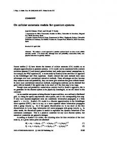
In this work, we consider a main road with 1000 cells, crossed by four other secondary roads to form a set of four junctions, each of them has it proper traffic light controller, as shown below :

Despite its simplicity, the NaSch model is capable of capturing some essential features observed in realistic traffic like density waves or spontaneous formation of traffic jams. To describe more complex situations such as multi-lane traffic, extensions of the NaSch model have been proposed where additional rules are added for lane changing cars [2-6].

Figure 1. The structure of our car traffic network

III. PROBLEM FORMULATION A. Traffic lights As mentioned previously, the aim of this paper is to propose a solution to have a flexible traffic light setting for improving the capacity of the system. To attain this goal, several strategies could be fixed. Minimizing total delay, as sum of all vehicles delays could be seen as an intuitive objective. Another goal is the maximization of the traffic flow. The minimization of the congestion (vehicles‘ number stops) is another objective to attain. In our case, we have chosen to minimize the total delay all over the network. Because of the complexity of the traffic network in a city, we adopt the same assumptions cited in [13] in order to simplify the problem: Only two light signals are considered: a green light and a red light. The duration of the red light Tr is equal to that of the green light Tg The cycle time T = Tg + Tr is the same for all lights.

All the roads in the system have a closed boundary condition; so that they behave as rings. The distances between the intersections are the same, and are equals to 250 cells. Each junction is assigned a number. Each number in a junction denotes the starting time of the green light in that junction. If S(u) denotes the starting time of the green light on a junction u, then (with the previous assumptions) the interval of the green light on u can be written as follow : [S(u) + kT, S(u) + kT + T/2 -1], where T denotes the cycle time and k an integer >=0. Since the crossing cell belongs to both roads, our model has to account for the fact that only one car may be in this intersection at one time. That is, during each time step, if the traffic light is red the vehicle approaching the junction, comes to a complete stop at the cell behind the crossing cell. At green light, the approaching vehicle progresses with respect to NaSch rules. However, at the end of the green phase some vehicles can occupy the crossing point. The stopped vehicle in the other direction, which is preparing to advance, must wait until the crossing cell becomes empty. Let d1 be the number of empty cells ahead between the vehicle and its leading vehicle. And d2 represents the number of empty cells ahead between the vehicle and the crossing point. We denote by pos the position of the crossing cell in the circuit. Then the second rule of the NaSch model becomes: If (the signal is red) then

gap = min (d1, d2) Else //the light is green If (a vehicle of a crossed road exists at pos) then gap = min (d1, d2) else gap = d1 end if End if V  min(V, gap – 1) Algorithm 1. The proposed Algorithm

B. Genetic algorithms Genetic algorithms (GA) attempt to mimic natural selection and Darwinian evolution. This approach developed by Holland [15], is used to treat several combinatory optimization problems. In these algorithms, a group of individual objects is given a task. The ones that perform the task the most efficiently are considered as the fittest. Just as in biological evolution where the fittest individual are the ones most likely to reproduce, genetic algorithms select the most fit objects and use them as templates to create a new generation of objects.

Vehicle

GA

Vehicle () accelerate () : void decelerate () : void randomization () : void motion () : void .... ()

- ... :

+ + + + + +

- population : Vector - .... :

*

1



Light

- .... :

*

+ Light () + .... ()

1

- .... : Road

Road () addVehicle () : void addLight () : void .... ()

Finally, each genetic algorithm needs stopped criteria. Generally, a genetic algorithm ends after a certain number of

+ + + +

The crossover consists in selecting two target individuals, denoted as parents, to generate two son individuals. The son‘s genes inherited either from one or other parent randomly. The process of our crossover consists of generating randomly a position in the two parents, and then permutes either the first parts in the two parent individuals, or the second parts. As in the mutation procedure, the crossover uses, generally, a probability pc between 0.5 and 0.9.

A class diagram in the UML language is a type of static structure diagram that describes the structure of a system by showing the system's classes, their attributes, and the relationships between the classes.

GA () selection () : Vector crossOver (String parent1, String parent2) : Vector mutation (String enfant) : String .... () : int

The next step is to explore the space of solutions. Starting from an initial population, generated previously, genetic algorithms explore the feasible set in order to generate new solutions using heuristic procedures. These new solutions are then evaluated. New solutions are produced by mutation and crossover operations. Mutation consists in selecting one individual and modifies one or more genes. How to modify the genes depends on the solution coding. Since our solution is formed by a sequence of numbers (each number represents the starting time of the green light of a junction) the mutation operation switches only one gene chosen randomly by another different number. Usually every existing solution is mutated with a very low probability pm, between 0.001 and 0.05.

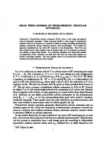
C. Object Oriented Modeling Before tackling the algorithmic part, it seems important to deal with the traffic network structure. For this, another requirement is important: the Object Oriented Modeling (OOM). The Object Oriented character of the designed model is very important, because we want to have the possibility of easy and half-automatic creation of the simulation program. The OOM also means that the simulation program should be divided into parts, representing urban traffic entities (road, vehicle, light …), that are connected together and the whole simulation is performed by communication among them. This Object Oriented Modeling (OOM) is realized with the Unified Modeling Language (UML).

+ + + + +

Genetic algorithms start from a feasible solutions subset. This subset is called the initial population, and is composed by r feasible solutions. Each solution, or individual, is described by its genes. In our case, an individual is formed with 4 genes. Each gene represents the starting of the green light at an intersection. Every individual is a specific signal setting. First of all, we start by generating randomly an initial population composed by r individuals. The evaluation of each solution is accomplished by the fitness function. The fitness function is the total delay on the network, which we want to minimize.

generations, but it can also end when a certain condition is reached, for example when the quality of an individual exceeds a certain threshold. In our case, the algorithm is stopped when certain number of iterations is reached.

Figure 2. The Object Oriented Modeling of our simulation program.

In the above figure, a road is made up of a set of traffic lights. A road is composed of one or more vehicles. This structure is better represented with a composition relationship, since the relationship between the ‗Road‘ class and the ‗Vehicle‘ class on one hand, and the ‗Light‘ class on the other hand represents a ‗part-whole‘ or ‗part-of‘ relationship.

IV. SIMULATION RESULTS AND ANALYSIS In the simulation, three methods for controlling the lights on the junctions are compared and analyzed. In the first method, we fix the starting times of the four traffic lights as, ‗0000‘, i.e. all the lights start at the same time. This method will be called ―synchronous timing method‖ (STM). In the second method, the system generates randomly four numbers representing the green time starts on the four junctions. We shall call this method as ―random timing method‖ (RTM). The third method is the ―genetic algorithm timing method‖ (GATM) which uses the genetic algorithms for generating a chromosome as a solution. Solutions are generated for each density value in order to minimize the total delay in the car traffic network. For the three methods, the randomization probability is assumed to be 0.3 in the NaSch model. The cycle time is equal to 6s. Initially, N cars are located randomly on the circuit (=1000 cells) and the velocity of each car is designated by an integer chosen from zero to the maximum vmax. The table 1 shows the parameters used in this work. Table 1. Parameters selected in the simulation.

Parameters of the model Length of each cell (m) Length of each car (cell) Total number of cells Maximum velocity (cell) Randomization probability

Value 7.5 1 1000 5 0.3

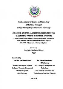
Figure 3 represents the simulation results. It shows the fundamental diagram (representing the global flow over the entire network) for the three methods previously cited, using the parameters listed in table 1. The cars density in each secondary road is fixed to 0.2, but the main road density is varied from 0.02 to 0.98. The data are collected after that time evolution reaches 1000 iterations.

methods. On the other side, the STM and the GATM have the same values of flows in the lower and medium density regions, but when the traffic density exceeds a critical value (about 0.6), the GATM is the most efficient method to enhance the flow. The observed phenomena could be analyzed as follows. For simplicity and without loss of generality; let us consider only two junctions in the system. For the RTM, it seems obvious. Indeed, since the beginnings of green lights in various crossing are generated randomly, they have not necessarily the same values ('03 ', '62', for example). This leads to asynchronous timing of lights in different crossings. We will distinguish two cases: the first value is less than the second, and otherwise. In the first case, '03 ', for example, a vehicle with a green light in the first crossing at time 0 will arrive at the second portion of the road where it will stop, either because the starting time of the second light is not yet reached, or because the second green light is switched on with a delay; causing therefore a formation of queues behind the crossing cell. In the second case, '62 ', for example, vehicles of the first junction are blocked while the second traffic light is green, and once vehicles of the first intersection are allowed to move (1st light is green), they will be blocked by the second traffic light. For STM, since the starting time of green lights has the same value, the lights are synchronized. When the lights are switched on, the vehicles moving downstream, find the road ahead free or less dense because the 2nd traffic light was green too. There is a synchronous traffic in the circuit. For the GATM, genetic algorithms seek a solution to minimize the waiting time. It is clear that the flow obtained in this case is optimal. On the other hand, Table 2 shows that when the density is less than 0.6 genetic algorithms often generate the solution '0000 '(about 60%), which justifies the fact that the results provided by the STM and the GATM are relatively identical for low and medium densities. For higher densities, the situation is more complicated. Indeed, because of the important number of vehicles, a fixed solution as ‗0000‘ is not always appropriate. Hence, the need for the genetic algorithm, that generates dynamically an adequate solution. This is illustrated in figure 3, where we show clearly that, at higher densities, only genetic algorithm can improve the traffic flow of the system. Table 2. Number of solutions generated by GA based on the density

Solution generated by GA 0000 Other than 0000

Density 0.6

35 24

6 53

V. CONCLUSION AND FUTURE WORKS Figure 3. The fundamental diagram for the three methods. Each point of the diagram represents the result from the latter 1000 iterations (to reach steady state) on a road of length 1000 starting from a random configuration.

From the figure 3, we can see clearly that the flow obtained with the RTM is very low compared with the two other

In this paper, we have shown that genetic algorithms could be used to provide an optimal solution to configure traffic light controllers in different junctions. The principal parameter adapted in this work is the starting time of green lights in each intersection. The simulation program we have constructed is

Object Oriented based. The program is designed with UML language and then implemented with Java language. It is, then, simple to understand and to modify to adapt it to others more complicated situations. Genetic algorithms used a roulette wheel selection, but other selection methods like, stochastic remainder without replacement selection or tournament selection could also be used. Thus, our first perspective here is to explore these methods and try to find the best one that suits our problem. Our next work will concern the optimization of the traffic light timing in more complicated traffic structure to model traffic in cities. Clearly our Object Oriented based implementation could easily adapt to this situation. Finally, we have combined genetic algorithms and the cellular automata with a view to design new traffic light controller software.

REFERENCES

1- K. Nagel and M. Schreckenberg, ―A cellular automaton model for freeway traffic‖, Journal of Physical I France, Vol. 2, pp. 2221-2229, 1992. 2- M. Rickert, K. Nagel, M. Schreckenberg, A. Latour, ―Two-Lane Traffic Simulations using Cellular Automata‖, Physica A: Statistical and Theoretical Physics, pp. 534-550, 1996. 3- P. Wagner, K. Nagel, D. E. Wolf, ―Realistic Multi-Line Traffic Rules for Cellular Automata‖, Physica A: Statistical and Theoretical Physics, pp. 687-698, 1997. 4- W. Knospe, L. Santen, A. Schadschnaider and M. Schreckenberg, ―Disorder effects in cellular automata for two-lane traffic.‖ Physica Journal A 265: Statistical and Theoretical Physics 265, pp. 614-633, 1998. 5- K. Nagel, D.E. Wolf, P. Wagner and P. Simon, ―Twolane traffic rules for cellular automata: A systematic approach‖, Physical Review E 58, American Physical Society, 1998. 6- N. Moussa and A.K. Daoudia, ―Numerical study of two classes of cellular automaton models for traffic flow on a two-lane roadway‖, Eur. Phys. J. B, vol. 31, no. 3, pp. 413-420, 2003. 7- R. Barlovic, L. Santen, A. Schadschnaider and M. Schreckenberg, ―Metastable states in cellular automata for traffic flow.‖ European Physics Journal, B 5, 793-801, 1998.

8- D. Chowdhury and A. Schadschneider, ―SelfOrganization of traffic jams in cities: Effects of stochastic dynamics and signal periods‖, Physical Review E, Vol. 59, No. 2, pp. R1311-R1314, Feb. 1999. 9- G. Bretti, R. Natalini, B. Piccoli, ―A Fluid-Dynamic Model on Road Networks‖, Arch Comput Methods Eng 139-172, 2007. 10- M. Caramia, C. D‘Apice, B. Piccoli, A. Sgalambro, ―Fluidsim : A Car Traffic Simulation Prototype Based on Flui Dynamic‖, Algorithms 2010, 3(3), 294-310; doi:10.3390/a3030294 2010 (www.mdpi.com/journal/algorithms) 11- A.Bradley, ―Design of an Intelligent Traffic Light System‖,http://www.tjhsst.edu/~rlatimer/techlab, 2004 12- G. Gentile, D. Tiddi ―Synchronization of traffic signals through a heuristic-modified genetic algorithm with GLTM‖, in proceedings of XIII Meeting of the Euro Working Group on Transportation, Padova University Press, Padua, Italy, ISBN 978-88-9035414-4 – 58 Syncronization GLTM (EWGT2009) 13- S. W. Chen, C. B. Yang and Y. H. Peng, ―Algorithms for the traffic light Problem on the Graph Model‖, http://par.cse.nsysu.edu.tw/~cbyang/person/publish/c0 7traffic.pdf 14- T. Kalganova, G. Russel and A. Cumming, ―Multiple Traffic Signal Control Using A Genetic Algorithm‖, SpringerWien New York, pp. 220-228, 1999. 15- J. H. Holland, ―Adaptation in Natural and Artificial Systems‖, Ann Arbor, University of Michigan Press, 1975.