Genetic Algorithm Optimized Neural Networks

Acta Chim. Slov. 2005, 52, 440–449 Scientiﬁc Paper

440

Genetic Algorithm Optimized Neural Networks Ensemble for Estimation of Mefenamic Acid and Paracetamol in Tablets Satyanarayana Dondeti,* Kamarajan Kannan, and Rajappan Manavalan Department of Pharmacy, Annamalai University, Annamalainagar, Tamil Nadu-608002, India. E-mail: [email protected]

Received 10-06-2005

Abstract Improvements in neural network calibration models by a novel approach using neural network ensemble (NNE) for the simultaneous Spectrophotometric multicomponent analysis is suggested, with a study on the estimation of the components of an analgesic combination, namely, Mefenamic acid and Paracetamol. Several principal component neural networks were trained with the Levenberg-Marquardt algorithm by varying conditions such as inputs, hidden neurons, initialization and training sets. Genetic algorithm (GA) has been used to develop the NNE from the trained pool of neural networks. Subsets of neural networks selected from the pool by decoding the chromosomes were combined to form an ensemble. Several such ensembles formed the population which was evolved to generate the fittest ensemble. Ensembling the networks was done with weighted average decided on the basis of the mean square error of the individual nets on the validation data while the ensemble fitness in the GA optimization was based on the relative prediction error on unseen data. The use of computed calibration spectral dataset derived from three spectra of each component has been described. The calibration models were thoroughly evaluated at several concentration levels using 104 spectra obtained for 52 synthetic binary mixtures prepared using orthogonal designs. The Ensemble models showed better generalization and performance compared to any of individual neural networks trained. Although the components showed significant spectral overlap, the model could accurately estimate the drugs, with satisfactory precision and accuracy, in tablet dosage with no interference from excipients as indicated by the recovery study results. The GA optimization guarantees the selection of best combination of neural networks for NNE and eliminates the arbitrariness in the manual selection of any single neural network model of a specific configuration, thus maximizing the knowledge utilization without risk of memorization or over-fitting. Key words: neural network ensemble, genetic algorithm, principal components, UV spectrophotometry, mefenamic acid, paracetamol

Introduction Neural Networks (NNs) of appropriate architecture have the ability to approximate any function to any desired degree. However, it has been shown that the transfer function must be continuous, bounded and non-constant for a NN to approximate any function.1 Fundamental background information on NNs can be found elsewhere.2–5 Research into the theoretical and practical aspects of the use of NNs for calibration and pattern recognition in analytical chemistry has increased rapidly in the last decade. Several papers employing neural networks have been published since then, in practically all areas of chemical research.6–11 There are some recent reports on the application of NNs for mixture analysis12–16 though most of them employ a separate network for estimation of each component and involves synthetic binary mixtures for calibration. Dondeti et al.

In NN based modeling, there are many degrees of freedom in selecting the network topology, training algorithm and training parameters. At the end of the training process, a number of trained networks are produced, and then typically one of them is chosen as best, based on some optimality criterion, while the rest are discarded.17 The present work, attempts to use the pool of trained networks (with potentially useful knowledge) to build an effective neural ensemble, which in consortium may be effective than single network models in terms of generalization and accuracy. Neural Ensemble: Neural network modeling essentially involves an optimization process by training a number of neural networks. Training the same model with the same training data set but with different initial environment, such as the initial weights, would end up in a slight different final sets of weights and hence the final performance.

Genetic Algorithm Optimized Neural Networks Ensemble

Acta Chim. Slov. 2005, 52, 440–449

441

are often used. Optimization is performed on a set of strings, where each string is composed of a sequence of characteristics. INITIAL POPULATION SELECTION

MATING

CROSSOVER

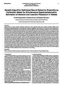
Figure 1. Graphical depiction of Neural Network Ensemble.

Therefore, one has to consider the intrinsic variance the NN models exhibit. An effective way of reducing the variance of the networks is to combine a number of networks to form an ensemble network.18 Neural network ensemble (NNE), shown in Figure 1, is a learning paradigm where a collection of a finite number of NNs is trained for the same task.19 It originates from Hansen and Salamon’s work20 which shows that the generalization ability of a neural network system can be significantly improved through ensemble of a number of neural networks, i.e. training many neural networks and then combining their predictions. The motivation for combining nets in redundant ensembles is that of improving their generalization ability. Combining a set of imperfect estimators can be thought of as a way of managing the recognized limitations of the individual estimators; each component net is known to make errors, but they are combined in such a way as to minimize the effect of these errors. Since this technology behaves remarkably well, recently it has become a very hot topic in both neural networks and machine learning communities.21 Genetic algorithms: Genetic Algorithms22 (GA) modeled on biological genetics and law of natural selection, operates by maintaining and modifying the characteristics of a population of solutions (individuals) over a large number of generations. This process is designed to produce successive populations having an increasing number of individuals with desirable characteristics. Like nature’s solution, the process is probabilistic but not completely random. The rules of genetics retain desirable characteristics by maximizing the probability of proliferation of those solutions (individuals) that exhibit them. GA operates on a coding of the parameters, rather than the parameters themselves. Just as the strands of DNA encode all of the characteristics of a human in chains of amino acids, so the parameters of problem must be encoded in finite length strings which might be a sequence of any symbols, though the binary symbols “0” and “1” Dondeti et al.

MUTATION

STOP?

NO

YES

END

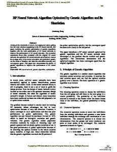
Figure 2. Typical GA.

Given an initial population of strings, a genetic algorithm produces a new population of strings according to a set of genetic rules. This constitutes one generation. The rules are devised so that the new generation tends to have strings that are superior to those in the previous generation, measured by some objective function. Successive generation of strings are produced, each of which tends to produce a superior population. Optimizing a population rather than a single individual contributes to the robustness of these algorithms. Any problem for which an objective function can be defined is a candidate for genetic optimization. A typical implementation of genetic algorithm is shown in Figure 2. For fundamental information on GA, one may refer to Goldberg.22 Scope of work: Given the wide-ranging applicability and uses of neural networks in the field of chemistry, improvements to the NN modeling process are highly desirable. In the process of NN modeling optimization several neural networks are trained with random initialization or with varying calibration data sets. Most of the knowledge of such network is discarded by employing only one network as calibration model. According to Chan et al.23 the generalization error of the ensemble network is generally smaller than that obtained by a single network while at the same time, the variance of the ensemble network is lesser than a single network, thus becomes a very effective way to improve the prediction ability. Motivated by these characteristics of NNE, and the earlier findings of the authors,24 the present study attempts to utilize a range of trained neural networks of varying configuration (in the number of hidden neurons) to form an effective ensemble employing the technique of Genetic


Acta Chim. Slov. 2005, 52, 440–449

442

Algorithms for the analysis of Mefenamic acid (MNA) and Paracetamol (PCM) combined tablet dosage used in the management of pain.

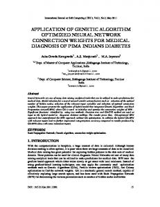
Experimental Chemicals and reagents: Analytical reagent grade NaOH was used to prepare 0.1M NaOH solution in distilled water which then served as a solvent for making the stock solutions and all further dilutions of MNA, PCM, their standard combinations and the tablet powder. Class A volumetric glassware such as pipettes and volumetric flasks were used for the purpose of making dilutions. Instruments and software: UV absorption measurements were carried out on PerkinElmer Lambda 25 double beam spectrophotometer controlled by UVWINLAB software version 2.85.04, using matched 1.00 cm quartz cells. All weights were measured on an electronic balance with 0.01 mg sensitivity. Spectra of all the solutions were recorded against a blank solution containing no analytes, between 200 to 400 nm and saved in ASCII format. Matlab® version 6.1 was employed for building Principal component LevenbergMarquardt neural networks (PCLMNN) and neural network ensembles. All computations were carried out on a desktop computer with a Pentium 4, 1.6 GHz processor and 256 MB RAM. Preparation of standard solutions: Standard solutions of pure MNA and PCM were made at different concentration levels ranging from 5 to 19 mg L–1 and 5 to 17 mg L–1 respectively for the purpose of linearity determination and to design the calibration data matrix from their spectra. The analytical levels of 10 mg L–1 and 9 mg L–1 respectively for MNA and PCM were chosen. The absorbance spectra, about the analytical level chosen for the two standards, are shown in Figure 3. 1.2

MNA PCM

1

Absorbance

0.8

0.6

0.4

0.2

0 220

240

260

280

300

320

340

360

380

400

Wavelengths (nm)

Figure 3. UV Spectra of Mefenamic acid and Paracetamol. Overlain spectra of MNA at concentration of 11.052 mg/L and PCM at concentration of 9.962 mg/L in 0.1M NaOH.

Dondeti et al.

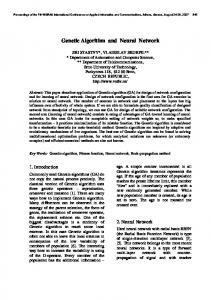
Calibration data: Since the absorbances were additive linearly in the desired range and no serious baseline problems or interactions were found in our trial studies in the desired range of concentration, the process described below was adopted in the design of calibration data set for training the PCLMNN. Three spectra of each component at three different concentration (low, medium and high) levels were employed in all possible combinations to provide a fair computation of calibration data set with some degree of experimental variation. A full factorial design was employed to obtain 49 training pairs from each spectral pair resulting in a total of 441 training pairs (49×9) representing the mixture space evenly with target concentrations that are orthogonal. A total of 441 training pairs thus obtained, constituting the complete calibration set, were used to train the PCLMNN model. All the target concentrations in the calibration set were then standardized (to a mean of 0 and standard deviation of 1). Spectral region between 220 and 340 nm was chosen on the basis of visual inspection of the spectra. Validation data: Randomized validation data sets were used for the internal validation and terminating the training of the PCLMNN at an optimum point to prevent over-fitting and retain generalization ability of the network. Validation data set of the same size was also designed from three different pairs of spectra of MNA and PCM standard out of which at least two pairs were different from that used in the calibration dataset. Synthetic binary mixtures for model evaluation: The synthetic binary mixtures were prepared on different days from fresh stock solutions of pure MNA and PCM, each day by separate weighing, in distilled water. Standard mixtures of the components were prepared with the concentrations lying within the known linear absorbance-concentration range by dissolving varying proportions of MNA and PCM stock solutions; the concentration of MNA varied between 50 to 175% of the test level concentration while that of PCM varied between 45 to 175% of its analytical level concentration. The concentrations of components were selected to span the mixture space fairly evenly, as show in Figure 4. Analysis of tablet dosage form: For the analysis of the active components of the analgesic tablet (Meftal Forte, MNA 500 mg and PCM 450 mg, Blue Cross Ltd., India, Batch No: HKF 333), twenty tablets were accurately weighed, carefully powdered and mixed. Tablet powder corresponding to the equivalent of 100 mg of MNA was dissolved in distilled water solution by sonication for 5 min and made up to 100 mL. The solution was centrifuged and 10 mL of supernatant was diluted to 100 mL to make a work dilution. 10 mL of work dilution was diluted to 100 mL to make the final solution. The final dilutions were made in two replicates from each


Acta Chim. Slov. 2005, 52, 440–449 18.000

T1 T2

PCM Concentration in mg / L

16.000

14.000

12.000

10.000

8.000

6.000

4.000 4.000

6.000

8.000

10.000

12.000

14.000

16.000

18.000

MNA Concentration in mg / L

Figure 4. Synthetic binary mixture design for testing the neural networks. Each point represents a mixture at the respective concentration of the components. The mixtures have been split in two groups T1 (ж) and T2 (◊). The design ensures that the model is thoroughly validated in a well distributed concentration space especially with regard to chosen analytical level. T1+T2=T.

work dilution, repeating the entire process for a total of 5 weights of the tablet powder. Each dilution was scanned in triplicate, each time for a fresh filling. For accuracy studies, by recovery, the same tablet powder was used in amounts corresponding to the equivalent of 55 mg of MNA (in order to enable spiking up to desired levels). The powder was then spiked with a known quantity of pure MNA and PCM and dissolved in 0.1M NaOH by sonication and the same dilutions as applied to tablet powder was done as explained above. A total of five powder samples were spiked to different levels in the range of 60 to 150%, each in two dilution replicates. PCLMNN model: Several PCLMNN models were built with varying number of input neurons (corresponding to the number of principal components chosen, viz. 2 to 4) and the number of hidden neurons. Principal component analysis was carried out by employing custom developed functions in MATLAB using the inbuilt Eigen value decomposition function (‘eig’) to obtain the latent (Eigen) vectors and the corresponding Eigen values. The scores obtained by projecting the standardized absorbance values on to these Eigen vectors were used as inputs. The PCLMNN had two neurons in the output layer corresponding to the two components of interest. The number of neurons in the hidden layer was varied from 2 to 5 neurons for each level of the input neurons chosen. The input layer and output layer nodes had identity and linear transfer functions respectively while the hidden layer nodes had sigmoid transfer functions for the PCLMNN, decided on the basis of earlier studies on neural calibration models.16,25,26 All the PCLMNN models were trained according to Levenberg-Marquardt27 algorithm available Dondeti et al.

in the neural network toolbox for MATLAB through the ‘trainlm’ function. The training was terminated when the validation performance as estimated by the mean square error (MSE), for a validation dataset, increased continually for more than 10 epochs since the last time it decreased. Three different calibration datasets were used for each given configuration and five replicate models obtained each with different initialization of weights by Nguyen-Widrow28 method. Neural Ensemble Model: A total of sixty PCLMNN models of selective configuration were used to build the Genetic Algorithm Optimized Neural Network Ensemble (GAONE). Three such models were developed by replicate runs of GA for each of the fitness dataset used. Weighted average based on the Mean Square Error (MSE) for the validation dataset of the respective PCLMNN model for each component formed the basis of combining the networks into an ensemble. Genetic Algorithm Implementation: Standard GA was employed using the Genetic Algorithm Toolbox29 for Matlab for the purpose of building the GAONE models. Binary coded chromosomes were employed with an initial population of 100. Fitness of the GAONE was estimated by determining the mean percentage relative prediction error (%RPE) of the GAONE for a fitness dataset (which was one of the test datasets from the spectra of binary synthetic mixtures) employed in the process. Roulette Wheel Selection schema was employed in determining the opportunities for individuals to reproduce and recombine to produce offspring. The rate of mutation was kept at the default level (0.7) provided by the GA Toolbox. Several GAONE models were developed from the base pool of 60 PCLMNN models by varying the fitness determining dataset (viz. test datasets T1 or T2) derived from the spectra of binary synthetic mixtures by repeating the GA process. Tablet analysis: Spectra recorded from the tablet solutions were analyzed by the GAONE calibration models and the concentrations predicted for each solution were used for calculation of the tablet content. Similarly MNA and PCM concentrations in the solutions prepared for recovery study were also obtained from the respective spectra and percentage recovery was calculated to determine the accuracy of the method.

Results and discussion The overlain absorption spectra in Figure 3 show extensive spectral overlap, which complicates the determination of the individual drug concentrations from a spectrum of a mixture. When considered separately, concentrations between 5 to 19 mg L–1 for MNA and 5 to 17 mg L–1 for PCM were studied and


443

Acta Chim. Slov. 2005, 52, 440–449

444

found to be linear over the space of 9 concentration levels (absorbances at 285 nm for MNA and 257 nm for PCM) with r2 of 0.9994 and 1.0 for each, slopes of 0.0408 and 0.0715, intercepts of 0.0049 and –0.0016 and residual standard deviation about the regression line being 0.0043 and 0.0018 respectively. There are many pitfalls in the use of calibration models, perhaps the most serious being variability in instrument performance over time. Each instrument has different characteristics and on each day and even hour the response may vary. Therefore it is necessary to reform the calibration model on a regular basis, by running a standard set of samples.30 Like other regression methods, there are constraints concerning the number of samples, which at times may be limiting the development of an ANN model. The number of adjustable parameters (synaptic weights) is such that the calibration set is rapidly over-fitted if too few training pairs are available leading to loss of generalization ability. Therefore, calibration sets of several hundred training pairs may often be necessary to get a representative distribution of the concentration across their range. This makes it expensive in time and resources to develop calibration mixtures physically in such large numbers which is rarely possible in routine laboratory studies and justifies our attempt to use mathematically constructed calibration data set from individual spectra of components. However, this approach cannot be applied in cases where significant non-linearity is exhibited. In general, a NNE is constructed in two steps, i.e. training a number of component neural networks and then combining the component predictions.31 For combining the predictions of component neural networks, the most prevailing approaches are plurality voting or majority voting 20 for classification tasks and simple averaging, weighted averaging17,32,33 that takes account of the relative accuracies of the nets to be combined or generalized ensemble method18 for regression tasks. Other possible methods such as correlation ensemble as suggested by Chan et al.23 where, the weighting of the ensemble was determined by the correlation of the output of the ensemble networks (Y) to the target output (X) as given by w=XTY, the more correlated is the network output, the higher the weighting value it has. In the present study weighted averaging was used. Several PCLMNN models in replicates were built as described in the experimental section by varying the calibration datasets, validation datasets, number of principal components and number of hidden neurons. The PCLMNN trained rapidly taking less than one minute and fewer than 300 epochs. PCLMNNs with an input of 3 neurons, an output of 2 neurons, both having linear transfer function and a hidden layer with 2 to 5 Dondeti et al.

neurons with sigmoid transfer function were chosen for building the GAONE models since they exhibited better performance in terms of the mean %RPE as shown in Table 1 and Figure 5. Mean Square Error ( MSE ) =

% RPE =

1 m 2 Σ1 (C act −C pred ) m

100 × MSE C

C act is the desired target, C pred is the output produced by the network for each input vector, C is the mean concentration of the component and m is the number of input vectors or samples. Twenty PCLMNNs were available for each of the calibration dataset from 5 replicate training for each configuration thus resulting in a base pool of 60 PCLMNNs from which ensembles could be built. Table 1. Optimization of PCLMNN models.

Indices

PCsa

1 2 3 4 5 6 7 8 9 10 11 12

2 2 2 2 3 3 3 3 4 4 4 4

Hidden Neurons 2 3 4 5 2 3 4 5 2 3 4 5

Mean %RPEb 2.2738 2.2705 2.2731 2.2862 1.5964 1.7092 1.9127 2.0719 2.5854 2.5912 2.9886 3.0780

a

Principal components used for the input. PCLMNN Models.

b

Standard Deviation 0.2473 0.2463 0.2475 0.2432 0.1396 0.1448 0.5135 0.3300 0.9591 0.9143 1.0360 1.2718 Average of 15

Though most ensemble approaches in engineering applications had been to employ all of networks available to constitute an ensemble, recently it has been reported that, ensemble of many of them may be better than ensemble of all the available neural networks.31 However, excluding those “bad” neural networks from the ensembles is not an easy task as we may have imagined. It is not as simple as combining few selected best performing networks, but combining networks that make error diversely, which as an ensemble perform better than any single NN in the population. Selection of nets for effective combination is to reduce the number of shared failures that a set of nets will produce. The extent to which they exhibit coincident failures can be determined only through a process of testing the performance of the selected ensembles.34 If there are N trained networks, the number of possible combinations would be 2N–1 which would be enormous as the value for N increases.


Acta Chim. Slov. 2005, 52, 440–449

Figure 5. Box-plot of the mean %RPE of 15 PCLMNN models for 12 neural network configurations. Refer to Table 1 for the respective configuration for each model index. The box has lines at the lower quartile, median, and upper quartile values. The whiskers are lines extending fro

It was reported that varying the data on which NNs are trained is more likely to result in a set of nets that can be combined more effectively than varying for instance the set of initial conditions from which they are trained, or topology.34 However, all approaches have been adopted in the present study as explained in section ‘Neural Ensemble Model’ using 60 PCLMNN models which formed the base pool. The possible combinations of NNs into ensemble equal 260–1 and hence the task of selecting the best one may be very intensive computationally. Hence GA approach was considered since they have been shown as a powerful optimization tool22 to pick the best ensemble from a pool of NNs with the use of a selection criterion. Genetic algorithms actively create a population of ensembles and search for the best ensemble which generalizes well.

The standard genetic operators, crossover and mutation, were used to create new individuals from an initial set. The fit members then form the next generation, and the process was repeated until a stopping criterion was reached. Genetic Algorithm Optimized Neural network Ensemble (GAONE) model development here was realized by utilizing the standard genetic algorithm22 with a binary coding scheme that represents each ensemble of neural networks. The process of coding and decoding the NNs that combine to form ensembles in the GA implementation is illustrated in Figure 6 using a single chromosome and for an assumed case of 20 models subset. An initial population 100 neural network ensembles were evolved by GA to build the GAONE model.

Figure 6. Coding and Decoding of Chromosome in building the GAONE Model.

Dondeti et al.


445

Acta Chim. Slov. 2005, 52, 440–449

446

In building ensembles the weighted average approach was preferred over the simple averaging because of the fact that one should believe accurate models than inaccurate ones. In this approach the predictions of the networks by taking a weighted sum of the output of each network, where each weight was based on the validation-set accuracy of the network. The present one being a multi-output case, an optimal combination of weights vector for each output were computed separately. The weights for combining the network in the ensemble was defined as follows (N equals the number of networks, ô be the ensemble output, wi, oi be the weight and output for the ith network): N

N

i =1

i =1

oˆ = � wi .oi with the constraint that � wi = 1 Mean square error (MSE) was chosen as the criteria for determining the weights in combining the NNs in to an ensemble since it is a measure of both the accuracy and variance. The exact mechanism of determination of weights in the present study is given below: Normalized MSE for each NN =

MSE Sum of MSE of All NNs in the NNE

Adjusted MSE for each NN = 1 − Normalized MSE for each NN

Combination Weights =

Adjusted MSE for each NN Sum of Adjusted MSE of all NNs in NNE

The selected NN models forming an individual (NNE) in the population were then combined on the basis of their MSE on their respective validation dataset employed while training as illustrated above. All the ensembles (individuals) thus formed were evaluated for their fitness using mean %RPE obtained for an unseen fitness dataset (T1, or T2). The individual having the lowest mean %RPE was considered the fittest individual and fitness ranking was assigned in the ascending order of mean %RPE. The parents were selected according to a probabilistic function (Roulette Wheel Selection) based on relative fitness. In other words, those individuals with higher relative fitness are more likely to be selected as parents. N children were created via recombination from the N parents. The N children were mutated and survive, replacing the N parents in the population. Mutation flips bits with some small probability (here it was 0.7), and is often considered to be a background operator. Recombination, on the other hand, was emphasized as the primary search operator. The GA was terminated when the highest ranking Dondeti et al.

individual’s fitness had reached a plateau such that 10 successive iterations were not producing better results (individuals) anymore. The process of building the GAONE models was repeated three times for each fitness datasets (T1 or T2). Many a times the GA found the same GAONE model (having the same constituent NNs) for a given fitness dataset in the replicate runs of GA. The performance was almost identical even when the constituent members varied. NNs with 2 to 5 hidden neurons were found in the ensemble working together in contrast to a single configuration chosen manually in NN models. The performance characteristics of the GAONE model are summarized in Table 2 and 3 for MNA and PCM respectively and the residual plots for the test dataset obtained from the binary synthetic mixtures (T, See Figure 4) are shown in figures 7a and 7b. Further GAONE model was employed in the analysis of tablets and the accuracy studies thereafter. Spectra obtained from 30 tablet solutions (including replicates) prepared from 5 different weightings as described in the experimental section were analyzed by the GAONE model (built from the entire pool of 60 PCLMNN models) and the average content was calculated. The results are summarized in Table 4. The accuracy of the method for analysis of tablets was further investigated using the recovery studies as described in the experimental section. The mean percentage recovery and its relative standard deviation obtained by the GAONE models for both MNA and PCM were found to be excellent as indicated in Table 5. Table 2. Mefenamic acid Prediction characteristicsa of GAONE calibration models.

Fitness Test Data %RPE Dataset Set T1 T (T1+T2) 1.530 T2 T (T1+T2) 1.525 T1 T2 1.129 T2 T1 1.872

Slope

Intercept Res.SDb

0.990 0.991 0.989 0.993

0.139 0.127 0.131 0.132

0.175 0.174 0.132 0.210

R2 0.998 0.998 0.999 0.997

a

Regression of the actual versus predicted concentrations. Residual Standard Deviation.

b

%

Table 3. Paracetamol Prediction characteristicsa of GAONE calibration models.

Fitness Test Data %RPE Dataset Set T1 T (T1+T2) 1.371 T2 T (T1+T2) 1.399 T1 T2 1.415 T2 T1 1.418

Slope 0.998 0.993 1.006 0.986

Intercept Res.SDb 0.051 0.127 –0.045 0.207

a

0.141 0.138 0.147 0.138

R2 0.999 0.999 0.998 0.999

Regression of the actual versus predicted concentrations. Residual Standard Deviation.


b

%

Acta Chim. Slov. 2005, 52, 440–449

447

Figure 7a. Residual plot obtained in the prediction of MNA from the synthetic binary mixtures (T) by GAONE model.

Figure 7b. Residual plot obtained in the prediction of PCM from the synthetic binary mixtures (T) by GAONE model. Table 4. Analysis of tablet samples by GAONE models.

Sample 1 (mg) Sample 2 (mg) Sample 3 (mg) Sample 4 (mg) Sample 5 (mg) Mean Tablet content (mg) Standard Deviation Relative Std Deviation Amount on the label (mg) % of the reported content a

MNA PCM GAONE-1a GAONE-2a GAONE-1a GAONE-2a 503.68 503.67 430.63 433.84 501.09 501.03 435.86 438.54 500.19 500.05 437.67 439.43 502.84 502.64 438.43 439.57 496.75 496.58 441.74 443.02 500.91

500.79

436.87

438.88

2.705

2.741

4.085

3.295

0.540

0.547

0.935

0.751

500.00

500.00

450.00

450.00

100.18

100.16

97.08

97.53

GAONE models obtained using different fitness datasets (T1 or T2).

Conclusions In developing neural network models for multivariate calibration, several networks are usually Dondeti et al.

Table 5. Recovery studies of MNA and PCM in tablets using the GAONE model.

Spiked Sample 1 2 3 4 5 Mean RSD

Mefenamic acid (MNA) Paracetamol (PCM) % Actual Found % Actual Found (mg) Recovery (mg) (mg) Recovery (mg) 70.42 72.92 103.55 62.28 62.33 100.08 80.03 82.36 102.91 71.24 71.70 100.65 106.31 107.31 100.94 95.60 94.77 99.13 132.03 132.48 100.34 119.48 118.18 98.91 155.86 155.06 99.49 141.70 139.18 98.22 101.45 1.701

99.40 0.970

trained since it is known that they exhibit intrinsic variance. Hence, retaining only one neural network model and rejecting others may not be good idea since many workers have found ensembles of neural networks as an effective way of reducing the variance, improving generalization and accuracy. Based on the reports that ‘many may be better than all’,31 the authors have earlier demonstrated that GAONE models were always better than any given single best neural network model or ensembles of all neural network models.24 The GAONE models developed in this study performed well in


Acta Chim. Slov. 2005, 52, 440–449

448

estimating MNA and PCM simultaneously when tested with spectra recorded on different days and exhibited ruggedness even when different sets of constructed calibration data were used in the model development as indicated by the prediction results. The accuracy of the GAONE model was also established in the analysis of the combined tablet dosage. The study indicates that in neural network calibration modeling, it may be worthwhile to build neural network ensembles having diversely configured neural networks than rely on an independent neural network model. May be, ‘working together works’, provided one is careful about who are working together.

Acknowledgements The authors grateful to the All India Council for Technical Education, New Delhi, for providing financial assistance under an R&D scheme to carry out this work. We are grateful MMC Health Care Ltd., Chennai, India for the generous donation of drug samples used in this study.

References 1. K. Hornik, Neural Netw. 1991, 4, 251–257. 2. S. Haykin, “Neural Networks - A Comprehensive Foundation”, Addison Wesley Longman, Singapore, 1999, pp 1–248. 3. L. Fausett, “Fundamentals of Neural Networks: Architectures, Algorithms and Applications”, PrenticeHall Inc, New Jersey, 1994, pp. 1–330. 4. R. J. Schalkoff, “Artificial Neural Networks”, McGraw-Hill Company, New York, 1997, pp. 1–182. 5. J. Zupan, J. Gasteiger, “Neural Networks in Chemistry and Drug Design”, Wiley-VCH, New York, 1999, pp. 1–154. 6. S. D. Brown, S. T. Sum, F. Despagne, B. K. Lavine, Anal. Chem. 1996, 68, 21R–61R. 7. B. K. Lavine, Anal. Chem. 1998, 70, 209R–228R. 8. J. Zupan, Acta. Chim. Slov. 1994, 41, 327–352. 9. J. Zupan, M. Novic, I. Ruisanchez, Chemom. Intell. Lab. Syst. 1997, 38, 1–23. 10. F. Despagne, D.L. Massart, Analyst [RSC, London], 1998, 123, 157R–178R. 11. S. Agatonovic-Kustrin, R. Beresford, J. Pharm. Biomed. Anal. 2002, 22, 717–727. 12. C. Yin, Y. Shen, S. Liu, Q. Yin. W. Guo, Z. Pan, Computers and Chemistry 2001, 25, 239–243. 13. Y. Ni, C. Liu, S. Kokot, Anal. Chim. Acta. 2000, 419, 185–196. 14. G. Absalan, M. Soleimani, Anal. Sci. 2004, 20, 879–882. 15. C. Balamurugan, C. Aravindan, K. Kannan, D. Sathyanarayana, K. Valliappan, R. Manavalan, Indian J. Pharm. Sci. 2003, 65, 274–278.

Dondeti et al.

16. D. Sathyanarayana, K. Kannan, R. Manavalan, Indian J. Pharm. Sci. 2004, 66, 745–752. 17. S. Hashem, Neural Networks 1997, 10, 599–614. 18. M. P. Perrone, L. N. Cooper, “When networks disagree: Ensemble methods for hybrid neural networks”, in: R. J. Mammone (Eds), Artificial Neural Networks for Speech and Image Processing, Chapman & Hall, New York, 1993, pp. 126–142. 19. P. Sollich, A. Krogh, “Learning with ensembles: how overfitting can be useful”, in: D. S. Touretzky, M. C. Mozer, M. E. Hasselmo (Eds), Advances in Neural Information Processing Systems, volume 8, MIT Press, Cambridge, MA, 1996, pp. 190–196. 20. L. K. Hansen, P. Salamon, IEEE Trans. Pattern Analysis and Machine Intelligence, 1990, 12, 993–1001. 21. A. J. C. Sharkey, “Combining artificial neural nets: ensemble and modular multi-net systems”, Springer-Verlag, London, 1999, pp. 1–30. 22. D. E. Goldberg, “Genetic Algorithm in Search, Optimization and Machine Learning”, Addison-Wesley, Reading, 1989, pp. 1–200. 23. L.-W. Chan, “Weighted least square ensemble networks”, in: Proceedings of the IEEE International Joint Conference on Neural Networks, Washington DC, 1999, 1393–1396. 24. D. Satyanarayana, K. Kannan, R. Manavalan, S. Afr. J. Chem. submitted for publication. 25. J. R. Long, V. G. Gregoriou, P. J. Gemperline, Anal. Chem. 1990, 62, 1791–1797. 26. D. Satyanarayana, K. Kannan, R. Manavalan, Acta Chim. Slov. 2005, 52, 138–144. 27. M. T. Hagan, M. B. Menhaj, IEEE Transactions on Neural Networks 1994, 5, 989–993. 28. D. Nguyen, B. Widrow, “Improving the learning speed of 2-layer neural networks by choosing initial values of the adaptive weights”, in: Proceedings of the International Joint Conference on Neural Networks, San Diego, CA, 1990, 3, pp. 21–26. 29. A. Chipperfield, P. Fleming, H. Pohlheim, C. Fonseca, Genetic Algorithm Toolbox, Version 1.2, Department of Automatic Control and Systems Engineering, University of Sheffield, England, 1994. 30. R. G. Brereton, Analyst (RSC), 2000, 125, 2125–2154. 31. Z.-H. Zhou, J. Wu, W. Tang, Artificial Intelligence 2002, 137, 239–263. 32. A. Krogh, J. Vedelsby, “Neural network ensembles, cross validation and active learning”, in: G. Tesauro, D. S. Touretzky, T. Leen, (Eds), Advances in Neural Information Processing Systems, Volume 7, MIT Press, Cambridge MA, 1995, pp. 231–238. 33. D. W. Opitz, J. W. Shavlik, Connection Science, Special issue on combining Artificial Neural: Ensemble Approaches, 1996, 8, 337–354. 34. A. J. C. Sharkey, N. E. Sharkey, G. O. Chandroth, Neural Computing and Applications, 1996, 4, 218–227.


Acta Chim. Slov. 2005, 52, 440–449

Povzetek Predlagamo izboljšave v umeritvenem modelu z uporabo ansamblov nevronskih mrež za multikomponentno spektrofotomoetrično analizo. Kot primer podajamo določitev analitov v mešanici mefenaminske kisline in paracetamola. Učenje nevronskih mrež smo dosegli z Levenberg-Marquardtovim algoritmom z različnimi začetnimi parametri, kot so začetni podatki, skriti nevroni, inicializacija in seti za učenje. Uporabili smo genetski algoritem za razvoj ansambla nevronskih mrež. Podsete nevronskih mrež, ki smo jih izbrali z dekodiranjem kromosomov, smo zbrali v ansamble. Več ansamblov je predstavljalo populacijo, iz katere se je razvil najboljši ansambel, optimizacijo pa smo izvedli na osnovi relativne napake napovedi. Opisujemo uporabo izračunanih umeritvenih setov spektrov iz treh spektrov posamezne komponente. Umeritvene modele smo evaluirali s pomočjo 104 spektrov 52 sintetičnih binarnih mešanic pripravljenih z uporabo ortogonalnega načrta. Modeli ansamblov kažejo boljše lastnosti kot katerakoli individualna nevronska mreža. Čeprav imajo analiti izrazito podobne absorpcijske spektre, jih lahko z zadovoljivo točnostjo in natančnostjo določimo v mešanicah v farmacevtskih pripravkih. Z uporabo genetskega algoritma omogočimo izbiro najboljše kombinacije nevronskih mrež in izključimo arbitrarnost ročne izbire.

Dondeti et al.


449