GENETIC ALGORITHM TOOLS FOR CONTROL SYSTEMS ...

GENETIC ALGORITHM TOOLS FOR CONTROL SYSTEMS ENGINEERING

A. J. Chipperfield, P. J. Fleming and C. M. Fonseca Department of Automatic Control and Systems Engineering, University of Sheffield, PO Box 600, Mappin Street, Sheffield, S1 4DU, UK INTRODUCTION

THE MATLAB GA TOOLBOX

There has been widespread interest from the control community in applying the Genetic Algorithm (GA) to problems in control systems engineering. Compared to traditional search and optimization procedures, such as calculus-based and enumerative strategies, the GA is robust, global and generally more straightforward to apply in situations where there is little or no a priori knowledge about the process to be controlled. As the GA does not require derivative information or a formal initial estimate of the solution region and because of the stochastic nature of the search mechanism, the GA is capable of searching the entire solution space with more likelihood of finding the global optimum.

Whilst there exist many good public-domain genetic algorithm packages, such as GENESYS [8] and GENITOR [9], none of these provide an environment that is immediately compatible with existing tools in the control domain. The MATLAB Genetic Algorithm Toolbox [10] aims to make GAs accessible to the control engineer within the framework of an existing CACSD package. This allows the retention of existing modelling and simulation tools for building objective functions and allows the user to make direct comparisons between genetic methods and traditional procedures.

GAs have been shown to be an effective strategy in the offline design of control systems by a number of practitioners. For example, Krishnakumar and Goldberg [1] and Bramlette and Cusin [2] have demonstrated how genetic optimization methods can be used to derive superior controller structures in aerospace applications in less time (in terms of function evaluations) than that of traditional methods such as LQR and Powell’s gain set design. Porter and Mohamed [3] have presented schemes for the genetic design of multivariable flight control systems using eigenstructure assignment, whilst others have shown how GAs can be used in the selection of controller structures [4].

MATLAB essentially supports only one data type, a rectangular matrix of real or complex numeric elements. The main data structures in the GA Toolbox are chromosomes, phenotypes, objective function values and fitness values. The chromosome structure stores an entire population in a single matrix of size Nind × Lind, where Nind is the number of individuals and Lind is the length of the chromosome structure. Phenotypes are stored in a matrix of dimensions Nind × Nvar where Nvar is the number of decision variables. An Nind × Nobj matrix stores the objective function values, where Nobj is the number of objectives. Finally, the fitness values are stored in a vector of length Nind. In all of these data structures, each row corresponds to a particular individual.

MATLAB has become a de-facto standard in Computer Aided Control System Design (CACSD) for the control engineer. The complete design cycle from modelling and simulation through controller design is addressed with a wide range of toolboxes, notably the Control System [5] and Optimization [6] Toolboxes, and the SIMULINK nonlinear simulation package [7] along with extensive visualisation and analysis tools. In addition, MATLAB has an open and extensible architecture allowing individual users to develop further routines for their own applications. These qualities provide a uniform and familiar environment on which to build genetic algorithm tools for the control engineer. This paper describes the development and implementation of a Genetic Algorithm Toolbox for the MATLAB package and provides examples of a number of application areas in control systems engineering.

Data Structures

Toolbox Structure The GA Toolbox uses MATLAB matrix functions to build a set of versatile routines for implementing a wide range of genetic algorithm methods. In this section we outline the major procedures of the GA Toolbox. Population representation and initialisation: crtbase, crtbp, crtrp The GA Toolbox supports binary, integer and floatingpoint chromosome representations. Binary and integer populations may be initialised using the Toolbox function to create binary populations, crtbp. An additional function, crtbase, is provided that builds a vector describing the integer representation used. Real-valued populations may be initialised using crtrp. Conversion

Presented at “Adaptive Computing in Engineering Design and Control”, Plymouth, UK, Spetember 21-22, 1994

between binary and real-values is provided by the routine bs2rv that also supports the use of Gray codes and logarithmic scaling. Fitness assignment: ranking, scaling The fitness function transforms the raw objective function values into non-negative figures of merit for each individual. The Toolbox supports the offsetting and scaling method of Goldberg [11] and the linear-ranking algorithm of Baker [12]. In addition, non-linear ranking is also supported in the routine ranking. Selection functions: reins, rws, select, sus These functions select a given number of individuals from the current population, according to their fitness, and return a column vector to their indices. Currently available routines are roulette wheel selection [11], rws, and stochastic universal sampling [13], sus. A high-level entry function, select, is also provided as a convenient interface to the selection routines, particularly where multiple populations are used. In cases where a generation gap is required, i.e. where the entire population is not reproduced in each generation, reins can be used to effect uniform random or fitness-based reinsertion [11]. Crossover operators: recdis, recint, reclin, recmut, recombin, xovdp, xovdprs, xovmp, xovsh, xovshrs, xovsp, xovsprs The crossover routines recombine pairs of individuals with given probability to produce offspring. Single-point, double-point [14] and shuffle crossover [15] are implemented in the routines xovsp, xovdp and xovsh respectively. Reduced surrogate [15] crossover is supported with both single-, xovsprs, and double-point, xovdprs, crossover and with shuffle, xovshrs. A general multi-point crossover routine, xovmp, that supports uniform crossover [16] is also provided. To support real-valued chromosome representations, discrete, intermediate and line recombination are supplied in the routines, recdis, recint and reclin respectively [17]. The routine recmut performs line recombination with mutation features [17]. A high-level entry function to all the crossover operators supporting multiple subpopulations is provided by the function recombin. Mutation operators: mut, mutate, mutbga Binary and integer mutation are performed by the routine mut. Real-value mutation is available using the breeder GA mutation function [17], mutbga. Again, a high-level entry function, mutate, to the mutation operators is provided. Multiple subpopulation support: migrate

The GA Toolbox provides support for multiple subpopulations through the use of high-level genetic operator functions and a function for exchanging individuals amongst subpopulations, migrate. A single population is divided into a number of subpopulations by modifying the data structures used by the Toolbox routines such that subpopulations are stored in contiguous blocks within each data element. The high-level routines, such as select and reins, operate independently on each subpopulation contained in a data structure allowing each subpopulation to evolve in isolation from the others. Based on the Island or Migration model [18], migrate allows individuals to be transferred between subpopulations. Uniand bi-directional ring topologies as well as a fully interconnected network are selectable via option settings as well as fitness-based and uniform selection and reinsertion strategies. EXAMPLE APPLICATIONS In this Section, three examples are used to illustrate a number of features of the GA that make it potentially attractive to the control engineer. The first example of the design of an aerospace control system demonstrates how GAs can be used to search a range of controller structures to satisfy a number of competing design criteria. The second example of nonlinear system identification shows how the GA confers an immediate advantage over conventional methods by allowing a choice of models to be made over a number of quality criteria. Indeed, this example presents a search method that has the potential to yield a more general approach to the system identification problem. The final example, from mixed-mode scheduling, illustrates a class of problems for which conventional search methods have been unable to yield optimal solutions. MIMO Controller Design This design example demonstrates how GAs may be used to select the controller structure and suitable parameter sets for a multivariable system. The system is a propulsion unit for an Advanced Short Take-Off, Vertical Landing (ASTOVL) aero-engine, shown in Fig. 1. It is required that the pilot have control of the fore-aft differential thrust (XDIFF) and the total engine thrust (XTOT). The inputs to the system are XTOTD and XDIFFD. The design problem is to find a set of pre-compensators that satisfy a number of time response specifications whilst minimizing the interaction between the loops. The time domain performance requirements, in response to a step in demand at one of the inputs, are (i) Maximum overshoot ≤ 10% (ii) 70% rise time ≤ 0.35 seconds (iii) 10% settling time ≤ 0.5 seconds

− +

1 XTOTD

KX(1)(s+KX(2)) (s+30) Lead−lag 1

+ +

Pre−compensator 1

1 0.025s+1 Actuator 1

+ +

+ +

1

XF/WFE

XTOT

KX(3)(s+KX(4)) (s+30) Pre−compesator 2 XR/WFE1

− +

+ + KX(5)(s+KX(6)) (s+30) Pre−compensator 3 2

+ −

XDIFFD

KX(7)(s+KX(8)) (s+30)

XF/A16 + +

Lead−lag 2 Pre−compensator 4

+ +

+ −

1 0.03s+1

2 XDIFF

Actuator 2

XR/A16

Figure 1: SIMULINK model of the ASTOVL propulsion unit. at the associated output. The amount of interaction, or cross-coupling, between modes is measured as ∞

∫ ( XTOT)

2

dt

0

when exited by a step input to XDIFFD, and vice-versa, and should be less than 0.05 for this design example. Thus, a total of eight design objectives must be satisfied. The ASTOVL propulsion unit is modelled directly in the SIMULINK package as shown in Fig. 1. To simplify the problem, pre-compensators are selected to be either first or second order or simple gains and pre-compensator parameters are represented using real values. Using a structured chromosome representation [19], it is possible to allow the free parameters for each possible precompensator to reside in all individuals, although only certain parameter sets are active in any given individual at any time. The active parts of a chromosome are controlled by high-level genes in an individuals representation. Thus, an individual may contain a number of possibly good representations at any time. In order to solve this problem using a simple GA, the design objectives are reformulated as a single minimax function thus:  F i − Goal i  f = max i  Goal i 

where Goali are the design goals and Fi are the individual objective functions associated with each design criteria. Using a population size of 40, the GA was run for 100 generations. A list of the best 50 individuals was continually maintained during the execution of the GA allowing the final selection of controller to be made from

the best structures found by the GA over all generations. XTOT/XTOTD

XTOT/XDIFFD

1.5

1.5

1

1

0.5

0.5

0

0

0.5 0

1

2

3

4

−0.5 0

1

XDIFF/XTOTD 1.5

1

1

0.5

0.5

0

0

1

2

3

4

3

4

XDIFF/XDIFFD

1.5

0.5 0

2

3

4

−0.5 0

1

2

Figure 2: Response of best ASTOVL controller found. Fig. 2 shows the response of the best controller found by the GA. In this case, all of the pre-compensator structures were of first order complexity and the design objectives where over obtained by a factor of 38.18%. The GA approach has the clear advantage over conventional optimization approaches in that it allows a number of controller structures to be examined in a single design cycle. The final choice of controller being made from a selection of different structures and parametric values. A minimax approach to this multiobjective problem has been described here that is simple to formulate and requires no special fitness assignment or selection methods. In other work [20], we have demonstrated the use of rank-based fitness assignment and niche induction techniques and shown how it is feasible to evolve populations of non-dominated solution estimates without having to combine individual design objectives.

Nonlinear System Identification Many problems in control engineering, signal processing and machine learning can be cast as a system identification problem. Here, the task is to determine a suitable model from a given set of input-output data. The resulting model can then be used for the prediction and control of a “blackbox” system. Whilst there are many tried and tested methods for linear system identification, in practice most real-world problems are nonlinear. The extra complexity associated with nonlinear system identification, particularly when there is no initial information or model structure detail, has to some extent contributed to the relative lack of attention to this particular field. This example illustrates a hybrid GA approach to the nonlinear system identification problem. Based on the NARMAX model (Nonlinear Auto-Regressive Moving Average model with eXogenous inputs), the GA is used to select a set of terms from a from a larger set of possible terms and lest-squares regression is used to find suitable parameter approximations. The NARMAX model for a SISO system is: y ( t ) = F( y ( t − 1 ) , …, y ( t − n y ) , u ( t − 1 ) , …, u ( t − n u ) , e ( t − 1 ) , …e ( t − n e ) ) + e ( t )

where y ( t ) , u ( t ) and e ( t ) represent the output, input and noise respectively and ny, nu and ne are the associated maximum lags. F is some, usually unknown, nonlinear function and {e(t)} is a zero mean independent noise sequence. Clearly, this can be written in the form of the linear regression model M

y ( t) =

∑ θi pi ( t) + ξ ( t) ,

t = 1, …, N

i=1

where N is the data length, pi(t) are monomials approximating F to a given order l and M is the number of distinct monomials. ξ is some modelling error and θi are the unknown parameters to be identified.

... pi(t) ...

i ...

...

The search for a suitable model structure can be regarded as a subset selection problem. Given a set of nonlinear terms, a model with a fixed number of terms is sought that minimises some criteria. Individuals are therefore subsets of the set of all feasible terms and are evolved to minimise the variance of the residuals associated with the model structure. index term 1 1 i1 i2 ... ik 2 y(t - 1) 3 y(t - 2)

N

u(t - nu)l

pi1(t)

pi2(t)

...

pik(t)

Figure 3: Chromosome coding: Models are represented as subsets with k elements.

Given the set of possible terms that the system may be constructed from, a look-up table may be used to map integers to model terms. Individuals are then composed of an unordered list of integers that represent potential model structures, see Fig. 3. The genetic operators used should guarantee that only valid models are produced, preferably without redundancy. Redundancy will exist when there are several different representations of the same model structure. A variation on the recombination operator proposed by Lucasius and Kateman [21] is used here. Offspring subsets are first produced from parents, preserving their intersection. The remaining elements are then shuffled and exchanged to produce two offspring. In this way, the order in which terms appear in parents is ignored and redundancy is eliminated (see Fig. 4). 6

4

7

3

1

9

5

1

2

4

4

1

7

3

6

1

4

2

5

9

4

1

7

5

9

1

4

2

3

6

(a)

(b)

(c)

Figure 4: Crossover: (a) Parents. (b) Retain common parts. (c) Cross. The mutation operator simply replaces terms in individuals with another term from the complimentary subset, Fig. 5. Thus, any mutated individual can be guaranteed to be valid. 6

8

3 4

1

7

5

15 9

13

10

11

14 12

2

16

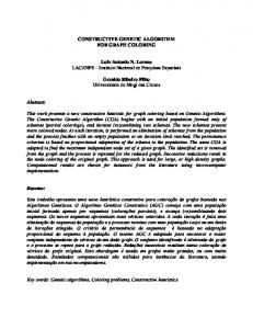
Figure 5: Subset mutation. The GA was applied to the identification of data obtained from a large pilot scale liquid level system with a zero mean Gaussian input signal. A model with 7 terms with degree l ≤ 3 and maximum lags nu = ny = 2 was assumed. The number of possible 7-term models is therefore 6724520. Using a population size of 40, the GA was run for 90 generations. The best 50 models evaluated on the basis of minimum residual variance over the entire search were maintained in a separate data structure to allow the comparison with other criteria after termination of the GA.

The performance of the best 50 individuals found is illustrated in Fig. 6 showing both residual variance and long-term prediction error. The points marked ⊕ correspond to the globally best solutions found in the sense that they minimize both performance measures simultaneously.

may be supplied by many others. A further simplifying assumption is that machines are connected in a strictly feed-forward structure. It is also assumed that input machines have an infinite resource available to them. A single machine is designated as the output machine and will not supply any other machines. Output from this machine is regarded as the output of the entire system.

0.06

Associated with each machine in the system is a control cost, Ci and a minimum Ti in which that machine may produce a unit of output. In many cases of interest this control cost can be considered to be strictly decreasing beyond Ti, for example when Ci is an integral cost function. From [22], the objective function to be minimised is:

1 0.05

0.045 2

3

0.04

N

f =

0.035

0.03 2.11

4

2.12

2.13 2.14 Residual Variance

2.15

2.16 -3

x 10

Figure 6: Performance of the 50 lowest variance models. Due to the subset selection method being a generate and test approach, the GA can produce a family of low variance models which may then be assessed according do different criteria before the final model is chosen. Additionally, searching in model space rather than term space has the potential to yield a more general approach to the system identification problem. Mixed-Mode Scheduling Here we consider a class of problems that, in general, have failed to yield to conventional search techniques. The particular problem that we will consider here is that of finding an optimal control strategy for a simple mixedmode system to produce K units of output in a fixed production time Tp for a minimum total control cost C [22]. Consider the system shown in Fig.7. 1 2

∑ Ci ( ti) ⋅ ( l + 1)

i=1

6

where ti ≥ Ti is the control time of machine i, N is the total number of machines in the system and l = K-1 is the number of units of output required subject to the constraint that the time to produce K units is less than Tp. A violation of this constraint invokes a penalty function which increases the value of the objective function proportionally with the level of violation. Again, a simple GA was used with a population of 40 individuals and run for 40 generations. The convergence of the optimization is shown in Fig. 8. These results are obtained from 10 independent runs and show the best worst and average performance at each generation. The sharp fall in the value of the fitness function is due to the constraint being satisfied. From Fig. 8 it can be seen that the GA consistently converges towards a minima. 3.9 3.8

Maximum Minimum Average

3.7 3.6 log10 * Fitness

Long-term Prediction Error

0.055

3.5 3.4 3.3 3.2 3.1

3

8

4 7

3 2.9 0

5

10

15

20

25 30 Generations

35

40

45

50

5 Figure 8: Convergence of the mixed-mode example. Figure 7: Simple mixed-mode system connection graph. Machines are connected in a network with the requirement that certain machines supply other machines with their output. For simplicity, we shall assume that machines supply at most one other machine although any machine

The same objective function was tested against a number of conventional optimizers, eg steepest-descent, BFGS, DFP and simplex. Only the simplex method was capable of finding a near optimal solution, and the quality of that solution was approx. 10% worse than those found by the GA. In addition, these search methods were also found to

be sensitive to the choice of initial estimates, a problem not encountered with the GA-based approach. CONCLUDING REMARKS We have presented a GA Toolbox for the CACSD package MATLAB and shown its application in a broad range of activities from control. Together with other control oriented toolboxes, the GA Toolbox provides a uniform environment for the control engineer to experiment with and apply GAs to problems in control. Whilst the GA Toolbox was developed with an emphasis on control engineering applications, it should prove equally useful in the general field of GAs as both a research vehicle and at the application level. ACKNOWLEDGEMENTS The authors gratefully acknowledge the support of this research by a UK SERC grant on “Genetic Algorithms in Control Systems Engineering” (GR/J17920). Carlos M. Fonseca would like to thank Programa CIENCIA, Junta Nacional de Investigação Científica e Tecnológica, Portugal, for their support. REFERENCES [1] Krishnakumar K. and Goldberg D. E., 1992“Control System Optimization Using Genetic Algorithms”, Journal of Guidance, Control and Dynamics, Vol. 15, No. 3, pp. 735-740, 1992. [2] Bramlette M. F. and Cusin R., “A Comparative Evaluation of Search Methods Applied to Parametric Design of Aircraft”, Proc. ICGA 3, pp213-218, 1989.

in Artificial Intelligence, Washington D.C., USA, 1990. [9] Whitley D., “The GENITOR algorithm and selection pressure: why rank-based allocations of reproductive trials is best,” in Proc. ICGA 3, pp. 116-121, 1989. [10] Chipperfield, A. J., Fleming, P. J., Pohlheim, H. and Fonseca, C. M., “A Genetic Algorithm Toolbox for MATLAB”, to appear in Proc. International Conference on Systems Engineering, Coventry, UK, 6-8 September, 1994. [11] Goldberg D. E., “Genetic Algorithms in Search, Optimization and Machine Learning”, Addison Wesley Publishing Company, January 1989. [12] Baker J. E., “Adaptive Selection Methods for Genetic Algorithms”, Proc. ICGA 1, pp. 101-111, 1985. [13] Baker J. E, “Reducing bias and inefficiency in the selection algorithm”, Proc. ICGA 2, pp. 14-21, 1987. [14] Booker L., “Improving search in genetic algorithms,” in “Genetic Algorithms and Simulated Annealing”, Davis L. (Ed.), pp 61-73, Morgan Kaufmann Publishers, 1987. [15] Caruana R. A., Eshelman L. A. and Schaffer J. D., “Representation and hidden bias II: Eliminating defining length bias in genetic search via shuffle crossover”, In Eleventh Int. Joint Conf. on AI, Sridharan N. S. (Ed.), Vol. 1, pp 750-755, Morgan Kaufmann, 1989. [16] Syswerda G., “Uniform crossover in genetic algorithms”, Proc. ICGA 3, pp. 2-9, 1989. [17] Mühlenbein H. and Schlierkamp-Voosen D., “Predictive Models for the Breeder Genetic Algorithm”, Evolutionary Computation, Vol. 1, No. 1, pp. 25-49, 1993. [18] Petty C. B., Leuze M. R. and Grefenstette J. J., “A Parallel Genetic Algorithm”, Proc. ICGA 2, pp. 155-161, 1987.

[3] Porter B. and Mohamed S. S., “Genetic Design of Multivariable Flight-Control Systems Using Eigenstructure Assignment”, Proc. IEEE Conf. Aerospace Control Systems, 1993.

[19] Dasgupta, D. and McGregor, D. R., “A Structured Genetic Algorithm: The Model and First Results”, Research Report IKBS-2-91, University of Strathclyde, UK, Sept. 1991.

[4] Varsek A., Urbacic T. and Filipic B., “Genetic Algorithms in Controller Design and Tuning”, IEEE Trans. Sys. Man and Cyber., Vol. 23, No. 5, pp1330-1339, 1993.

[20] Fonseca C. M. and Fleming P. J., “Genetic Algorithms for Multiple Objective Optimization: Formulation, Discussion and Generalization”, Proc. ICGA 5, pp. 416-423, 1993.

[5] Grace A. C. W., Laub A. J., Little J. N. and Thompson C., “Control System Toolbox User’s Guide”, The MathWorks, Inc., 21 Eliot St., South Natick, MA 01760, 1990.

[21] Lucasius and G. Kateman, “Towards Solving Subset Selection Problems with the Aid of the Genetic Algorithm”, PPSN 2, pp239-247, 1992.

[6] Crummey T. P., Farshadnia R., Fleming P. J., Grace A. C. W. and Hancock S. D., “An Optimization Toolbox for MATLAB”, Proc. IEE Control ’91, Edinburgh, UK, Vol. 2, pp744-749, 1991. [7] Grace A. C. W., “SIMULINK, an Integrated Environment for Simulation and Control”, In, “MATLAB Toolboxes and Applications for Control”, Chipperfield A. J. and Fleming P. J. (Eds.), Peter Peregrinus, 1993. [8] Grefenstette J. J., “A User’s Guide to GENESIS Version 5.0”, Technical Report, Navy Centre for Applied Research

[22] Banks, S. P. and Yang, Y. Y., “Optimal Strategies for a Simple Mixed-Mode System”, Proc. European Simulation Multiconferrence, Barcelona, June 1-3, 1994.