Characterizing the Genetic Programming Environment for FIFTH (GPE5) on a High Performance Computing Cluster Kenneth Holladay Southwest Research Institute San Antonio, Texas
[email protected] ABSTRACT Solving complex, real-world problems with genetic programming (GP) can require extensive computing resources. However, the highly parallel nature of GP facilitates using a large number of resources simultaneously, which can significantly reduce the elapsed wall clock time per GP run. This paper explores the performance characteristics of an MPI version of the Genetic Programming Environment for FIFTH (GPE5) on a high performance computing cluster. The implementation is based on the island model with each node running the GP algorithm asynchronously. In particular, we examine the effect of several configurable properties of the system including the ratio of migration to crossover, the migration cycle of programs between nodes, and the number of processors used. The problems employed in the study were selected from the fields of symbolic regression, finite algebra, and digital signal processing.
Categories and Subject Descriptors I.2.2 [Artificial Intelligence]: Automatic Programming – Genetic Programming, High Performance Computing
General Terms Performance, Experimentation, Languages
Keywords Genetic Programming, High Performance Computing, Digital Signal Processing
1. INTRODUCTION Introduced in 2007 [7], the Genetic Programming Environment for FIFTH (GPE5) incorporates several important features that set it apart from other genetic programming (GP) systems. GPE5 programs are evolved using a stack-based language (FIFTH) whose syntax and interpreter is similar to FORTH. The single parameter stack for FIFTH holds containers that support multiple data types with intrinsic handling of vectors and matrices. Other
Permission to make digital or hard copies of all or part of this work for personal or classroom use is granted without fee provided that copies are not made or distributed for profit or commercial advantage and that copies bear this notice and the full citation on the first page. To copy otherwise, or republish, to post on servers or to redistribute to lists, requires prior specific permission and/or a fee. GECCO’09, July 8–12, 2009, Montréal Québec, Canada. Copyright 2009 ACM 978-1-60558-325-9/09/07...$5.00.
stack-based GP languages such as PUSH3 [14] use separate stacks for each data type with no provision for manipulating a vector as an object. FIFTH is expressive and easily extensible. In addition to the typical math and logic functions, the operators include high level vector transforms (e.g., windowing and Fourier transform) as well as vector reductions (e.g. mean, standard deviation, and variance). GPE5 includes a FIFTH interpreter, allowing generated programs to be embedded directly into applications. A second distinguishing feature is that GPE5 uses a linear program representation (instead of a tree) and performs all evolutionary manipulations using stack, branch, and flow control tracing to ensure both syntactic and operational correctness. While there have been other published efforts using stack tracing [15], GPE5 is the first publicly available code set to do so. These features enable GPE5 to solve classes of problems in areas such as digital signal processing that were previously intractable to GP techniques [8]. The initial design of GPE5 recognized the benefit of utilizing multiple processors to solve practical problems within reasonable time periods. The implementation was based on a distributed design with the Common Object Request Broker Architecture (CORBA) as the inter-process communication middleware. A single master node performed all of the genetic manipulation functions while the more time consuming fitness evaluations were distributed over available computing resources. The code base proved to be robust for heterogeneous groups of computers (mixtures of Windows, Linux and Sun operating systems) connected in a local area network, and it exhibited reasonable scaling efficiency for small numbers of computers. However, vector based signal processing problems often required days of wall clock time to complete a single run even when using up to 30 processors. It was clear that achieving a meaningful reduction in the wall clock time consumed to solve complex problems would require a significant increase in computing resources, such as those available on a High Performance Computing (HPC) cluster. This paper describes the process of creating a Message Passing Interface (MPI) version of GPE5 to run on the Lonestar system at the Texas Advanced Computing Center (TACC). TACC is part of the National Science Foundation’s TeraGrid project. Section 2 gives a summary of the technical approach used to port the software, as well as a description of the configuration parameters unique to the parallel implementation of GPE5. Section 3 introduces the experimental problems used to measure performance and the results for each problem. The final section discusses the practical implications of the work.
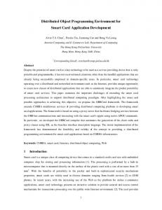
2. TECHNICAL APPROACH The distributed architecture of the CORBA version of GPE5 is not well suited to parallelization, as many of the processors are idle during the genetic manipulation process. When creating parallel versions of serial programs, using more resources is only effective if the computational work can be divided evenly among the available processors. Fortunately, the GP literature describes multiple techniques for creating parallel versions of genetic programming algorithms, typically achieving linear or super-linear performance[1]. While recent publications have shown interesting results using the finegrained model [6] and cooperative co-evolution model [11], we chose to implement a variation of the course-grained or island model [5] to minimize the necessary code changes. In the island model, every processing node runs the same GP algorithm performing both genetic manipulation and fitness evaluation on its own private population known as a deme. Since CORBA is not typically supported for parallel applications on HPC platforms, the more common Message Passing Interface (MPI) [12] was selected for interprocess communication. An important goal of the software conversion work was to achieve a code base that could be compiled on multiple operating systems (Windows, Linux, Sun) and produce three GPE5 applications: a distributed version using CORBA, a stand-alone version for a single computer, and a parallel MPI version. The first step in accomplishing these objectives was to restructure the code base to abstract the CORBA communication, thus decoupling the communication requirements from the genetic programming logic. This resulted in a FIFTH library containing all of the core GP components including the FIFTH interpreter, data set management, population management, fitness calculation, and genetic manipulation. The library consists of approximately 20,000 lines of code in 45 files. The reconstructed CORBA version required 11 additional files containing about 3,000 lines of code. After completing the code refactoring and abstraction, a stand-alone version of GPE5 was created by adding a single file with less than 800 lines of code. As illustrated in Figure 1, the architecture for the MPI version (MGP5) centers around three new classes: GPRun (control logic for the GP algorithm), Receiver (accepts all incoming MPI messages), and Sender (handles all outgoing MPI messages).
Two key design choices resulted in a clean and easily extensible implementation comprised of only 1100 lines of code in 7 files. First, the multi-threaded version of the MPI library allows the Sender and Receiver to operate asynchronously while using the synchronous MPI_Send() and MPI_Recv() calls. Second, all messages between nodes are formatted in XML. Our version of the island model required only one new configuration parameter. The serial version of GPE5 already had a parameter to specify how many of the top ranking programs were copied (migrated) into the next generation. For the parallel version, this becomes the number of programs to send to neighboring nodes. A new “Cycle” parameter controls how often programs are sent. A Cycle value of 0 means that no programs are exchanged, a value of 1 sends programs at the end of every fitness evaluation cycle, a value of 2 every other cycle, and so forth. The computing nodes are considered logically connected in a toroidal grid so that each node has four neighbors. After genetically manipulating one generation to produce the next generation, the GPRun class checks the received program queue to determine whether any new programs have arrived from one or more of its neighbors. If so, all programs are removed from the queue and are added to the next generation before executing the fitness evaluation cycle. This method allows each node to progress through generations at an independent rate. Node 0 has two unique responsibilities. First, it writes three summary reports at various stages in response to messages from the other nodes. These include a record of when each node found its first fit entry, an intermediate indication of the number of evaluations performed, and a brief summary generated during the shutdown process. Second, node 0 ensures a clean termination for all nodes. When any node meets the termination criteria (fitness, minimum generations, maximum generations, etc.) it sends a Done message to node 0. Node 0 then sends a Quit message to all other nodes, causing them to send their Done messages. Once node 0 receives a Done message from each of the other nodes, it sends out a Shutdown message causing all nodes to terminate. All development and testing of MGP5 occurred on the Lonestar Dual-Core Linux Cluster which is configured with 5,200 compute-node processors, 10.4 TB of total memory and 95 TB of local disk space. The peak performance is rated at 55 TFLOPS. Nodes are interconnected with InfiniBand technology in a fat-tree topology with a 1GB/sec point-to-point bandwidth. Jobs are submitted using the LSF batch system. Turn around time for a job ranges from a few minutes to a few days, depending on the resources requested (number of processors and estimated wall clock time) and system utilization. The complete source code for all versions of GPE5 is available at fifth.swri.org.
3. EXPERIMENTS AND RESULTS
Figure 1 - Class diagram of the MPI logic and control portion of MGP5.
Characterizing the performance of a GP system is a difficult task. While there are many test problems that have been published by GP researchers, there is no well-recognized test suite. Many researchers choose one or more of the problems introduced by Koza [9, 10] such as Boolean multiplexers, Boolean parity, Lawnmower, Bumblebee, or others. A previous empirical study of the parallel performance of an island model, tree-based GP system [4], used even parity 4, artificial ant, and symbolic
regression. As noted by Daida [3], a general theme is to include one problem each from the categories of Boolean logic, symbolic regression, and finite state machine. Rather than follow this trend for our initial characterization of MGP5, we decided instead to choose problems that differed significantly in three key areas that affect performance: data set size and type, operator selection and complexity, and expected problem difficulty. Problem difficulty is a comparison based on measurements from trial runs with the serial version of GPE5 and includes both an estimated probability of success (POS) and the average wall clock time consumed. The three selected problems are taken from symbolic regression, finite algebra, and digital signal processing.
3.1 Symbolic Regression One of the most common real-world applications of GP is finding a mathematical model that fits a specific data set. In GP literature, this is often referred to as symbolic regression. We selected the binomial-3 problem for the first set of experiments. For a detailed analysis of the characteristics of this problem that make it popular for GP studies, see [2]. The model is expressed formally as:
f ( x ) (1 x )
3
3.1.3 Operators and Terminals The set of operators was limited to primitive math (*/+-). The only input terminal was the abscissa value (x). GPE5 has a different approach to ephemeral random constants (ERCs). The configuration file specifies a set of values that may be randomly selected by the program builder and genetic operators. We have found that using a small set of prime numbers often works well as the programs evolve their own combinations to produce values in . For this problem, we included 1, 2, 3, 5, 7, 11, -1.
3.1.4 Problem Difficulty Test runs with this problem rank it as relatively easy. Using a population size of 1000 programs per generation, POS for a serial run is about 80% within 20 generations with an average time expenditure of about 7 seconds per generation.
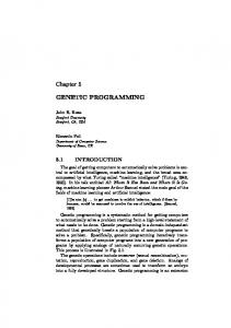
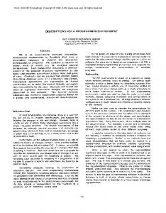
3.1.5 Experiments and Results The first set of experiments used a migration cycle of zero and 128 processing nodes. The purpose was to characterize a baseline performance and determine the effect on POS when varying the probability of mutation (M) and crossover (X) during genetic manipulation. Figure 3 shows the results. 1
3.1.1 Data Set
400
f(x)
200
0.8 Probability of Success
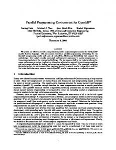
The generated data set contains 500 points evenly spaced over the interval [-6, 6], which includes the inflection point (Figure 2). This is a moderate number of points that are easily kept entirely in memory. For each generation evaluation, the data set manager used 50 points, seven of which were common for all generations and 43 of which were randomly selected.
0.6 M=0.0 X=1.0 M=0.2 X=0.8
0.4
M=0.8 X=0.2 M=1.0 X=0.0
0.2
0
0 -200
-5
0 x
5 3
3.1.2 Fitness Program fitness (fp) was calculated as the mean of the difference between the program output (pi) and the known desired output (oi) over the number of data points used (n). This provides a high resolution, continuous function with a value of zero being a perfect fit. The fitness target was set to 0.0001.
fp
1 pi oi n i 1
20
40 Generation
60
80
Figure 3 - Effect of mutation (M) and crossover (X) on the probability of success for the polynomial regression problem.
Figure 2 – Graph of the function f ( x ) (1 x ) .
n
0
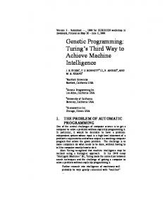
The highest POS is achieved using a mutation probability of 0.8 and a crossover probability of 0.2. Therefore, these probabilities were used in the second set of experiments to characterize the effect of the migration cycle. Still using 128 processing nodes per run, Figure 4 shows the improvement in the POS as the migration cycle is decreased from 4 to 1, effectively achieving a 100% probability of solution in less than 10 generations. We selected a migration cycle of 2 for the final experiment. The final experiment was designed to indicate the effect of the number of processors on the wall clock time required to achieve a solution while performing approximately the same amount of work during each run. Using the total number of programs evaluated in a generation across all nodes as a rough estimate of
the work expended, we selected a baseline of 128,000 (product of the number of nodes and the population size per node). This approach has an obvious scalability problem since at some point the number of programs per node will drop to a critical level below which genetic manipulation will not be effective. Table 1 shows the timing results for four representative runs. The Resource Seconds column is the time charged by the batch system for the run (the elapsed wall clock time multiplied by the number of processing nodes used) and is thus a real measure of the resources consumed. Note that increasing the number of processors from 16 to 128 results in a 32% reduction in resource consumption and an 84% reduction in wall clock time. Moving from 16 to 256 processors actually increases the resource consumption by 8%, but results in a 92% reduction in wall clock time. While 84% and 92% sound impressive, they equate to only 2.5 and 2.8 minutes respectively.
Table 2 – Single operator results for three element algebra A1. $
0
1
2
0
2
1
2
1
1
0
0
2
0
0
1
The data set for this problem poses some unique challenges. Since it consists of all possible combinations of the three element grammar, it contains only 27 entries. This is a small number of test cases relative to the number of terms in the expected output. In addition, the result of a normal error calculation, such as that used in the polynomial regression problem, does not convey a distance meaning. That is, an output of 0 when it should be 2 (error = 2) is really no worse than an output of 1 when it should be 2 (error = 1).
0.8 Probability of Success
Using a dollar sign to represent the operator, Table 2 shows the single operator grammar for the three element algebra A1. The aspects of this problem that make it an interesting candidate for GP study are detailed in the following subsections.
3.2.1 Data Set
1
0.6
0.4
0.2
C=1
3.2.2 Fitness
C=2
This type of problem is well suited to the “percent incorrect” fitness evaluation available in GPE5. The calculated answer is deemed to be correct if it is within a specified tolerance (τ) of the actual output. We used τ =0.01. The fitness function is:
C=4 C=0
0
x if x y t A ( x, y , z ) z if x y
0
20
40 Generation
60
80
Figure 4 - Effect of migration cycle (C) on the probability of success for the polynomial regression problem. Table 1 - Parameters and results for varying number of nodes applied to the polynomial regression problem. Nodes Per Run
Programs Per Node
Seconds to Solve
Resource Seconds
fp
100 n pi oi n i 1
While this eliminates the distance measure ambiguity, it exposes a dangerous limitation. With only n=27 points to evaluate, the fitness result can only take on 27 discreet values. This is a very low resolution, effectively providing only 27 bins into which the programs for each generation would be sorted. However, the effective resolution for GPE5 will be somewhat better. When sorting programs, if the fitness of two programs is identical, the fitness of the shorter program is considered better.
16
8000
182.5
6,611.1
64
2000
42.4
5,636.1
3.2.3 Operators and Terminals
128
1000
28.7
4,436.9
The terminals for this problem are x, y, and z.
256
500
14.4
7,178.0
This problem requires only a single operator, but since it is not a standard math or logic operator, it would have to be coded into most GP systems. However, with GPE5, the configuration file allows the specification of pre-code that is executed prior to the program and which is neither included in the program length nor used in the genetic manipulation operations. That capability allowed us to define the $ operator in FIFTH as follows:
3.2 Finite Algebra The second problem selected for study comes from the field of finite algebra. Spector [13] introduced this problem to GP researchers in 2008, demonstrating outstanding results where GP solutions were significantly better than human solutions. For this study, we selected the search for a discriminator operation using Spector’s A1 grammar. The discriminator operation on algebra A is given by:
{ 2 1 2 | 1 0 0 | 0 0 1 } CONSTANT A1 VARIABLE aTable A1 aTable ! WORD $ SWAP HORZCAT aTable SWAP {}@ ENDWORD
3.2.4 Problem Difficulty With its small memory footprint and minimal number of operators and terminals, this problem might appear trivial. However, test runs rank it as moderately difficult. Using a population size of 1000 programs per generation, POS for a serial run is less than 5% within 400 generations with an average time expenditure of about 6 seconds per generation.
generations. This does not represent the best solution of which GPE5 is capable. These studies were constructed to measure the time to the first correct solution. While the GPE5 configuration can be set to continue processing after reaching a solution (as long as fitness continues to improve), this potential improvement requires additional time and resource consumption. 1
The best 100% correct discriminator term for algebra A1 reported by Spector required 3,210 generations and contained 39 terms. With that as a basis, we constrained the program size to be between 5 and 200 terms.
Figure 5 shows the effect on POS with constant migration cycle (C=0) and processing nodes (n=128) while varying the probability of mutation (M) and crossover (X). Although the lines are rather cramped, the M=0.8 and X=0.2 values perform marginally better. 1
Probability of Success
3.2.5 Experiments and Results
0.8 C=1 C=2 C=10
0.6
C=0
0.4
0.2
M=0.0 X=1.0 M=0.2 X=0.8 M=0.8 X=0.2
Probability of Success
0.8
0
M=1.0 X=0.0
0
100
0.6
200 Generation
300
400
Figure 6 - Effect of migration cycle for the A1 grammar discriminator problem. 0.4
Table 3 - Parameters and results for varying number of nodes applied to the finite algebra problem.
0.2
0
Nodes Per Run 0
100
200 Generation
300
400
Figure 5 - Effect of mutation and crossover probabilities for the A1 grammar discriminator problem. Figure 6 shows the dramatic effect on POS of varying the migration cycle. Note that migrating programs between nodes every generation (C=1) did not perform as well as migrating every 2 generations (C=2). In fact, several runs with C=1 failed to produce any fit programs within 500 generations. With C>=2, the POS generally improved with lower values of C. The final experiment runs used C=2. The final experiment to determine the effect of the number of processors on the wall clock time required to achieve a solution used the same constant work premise basis of 128,000 evaluations as the theoretical total per generation. Table 3 shows the timing results for four runs. For this problem, the resource reduction decreased with every increase in the number of processors. Increasing from 16 to 256 processors reduced the wall clock time by 97% (35.7 minutes). The best 100% correct discriminator program produced during these experiments contained 102 terms and was found in 72
Programs Per Node
Seconds to Solve
Resource Seconds
16
8000
2,196.4
38,562
64
2000
435.2
31,101
128
1000
107.8
17,666
256
500
53.6
17,545
3.3 Digital Signal Processing The final problem addressed in this paper comes from the field of digital signal processing. This is a feature extraction task where the goal is to evolve an algorithm that highlights symbol transitions in a digital signal so that the symbol rate (baud) can be easily calculated. The output of the evolved program is expected to be a vector that if plotted would show significant peaks or valleys at the majority of the symbol transitions. The output vector is post processed using Fourier analysis to determine the symbol rate. To avoid having to write special code and compile it into GPE5, the post processing algorithm can be written in FIFTH and included in the problem configuration file as follows: WND_HAMMING FREQCOMP VMAXINDEX x LENGTH SWAP DROP Fs SWAP / * symbolsPerSec .
. " ," .
This code expects an output vector on the stack. The symbol x is the signal vector, and Fs is the sampling frequency. The code extracts the frequency components, locates the maximum peak, and converts the peak index into a symbol rate. The result consists of two values required by the fitness calculation: the calculated symbol rate and the actual symbol rate. A complete description of the symbol rate problem may be found in reference [8].
significant than the absolute error. For example, a 10 baud error when the actual rate is 50 baud represents a much more significant inaccuracy that if the actual rate is 2400 baud. The relative error fitness function in GPE5 is defined as:
fp
1 n pi oi n i 1 oi
3.3.1 Data Set Symbol rate estimation typifies a large class of DSP problems where the raw data is best represented as a vector. This makes the data set management significantly more complicated than the previous problems. The first step is to create a collection of signals that adequately represents the domain of interest. Table 4 lists common signal, channel, and receiver properties that affect the performance of blind symbol rate estimation algorithms for surveillance systems working in the High Frequency (HF) range of 3-30 MHz. The last column indicates the range of values used in this experiment for each property. Table 4 - Properties of the training set signals used for the symbol rate experiments. Property Modulation
Typical values in HF FSK, MSK, PSK, DPSK, OQPSK, QAM, ASK
3.3.3 Operators and Terminals Table 5 lists the terminals and operators used for this problem along with the probability of selection during initial random program generation and mutation. The last row includes a number of vector transformation operators, both general and domain specific. Table 5 – Terminals and operators used for the symbol rate problem. Terminals and Operators
Probabilit y of selection
Values used
X
0.1
FSK, PSK
1, 2, 3, 5, -1, PI
0.1
+ - * /
0.1
REAL IMAGINARY ANGLE UNWRAP MAGSQRD MAGNITUDE DIFF FFT SQRT VRAMP ROUND REVERSE COS SIN WND_HAMMING FLOOR CEILING
0.7
Pulse shape
None, raised cosine (RC), root RC (RRC), Gaussian
None, RC
Excess bandwidth (rolloff)
Limit: 0.00 to