Proceedings of the International Multiconference on Computer Science and Information Technology pp. 437–446
ISSN 1896-7094 c 2007 PIPS
Genetic Programming for Dynamic Environments Zheng Yin1 , Anthony Brabazon1, Conall O’Sullivan2 , Michael O’Neill1 1
Natural Computing Research and Applications Group University College Dublin, Ireland.
[email protected] [email protected] [email protected] 2 School of Business, University College Dublin, Ireland.
[email protected]
Abstract. Genetic Programming (GP) is an automated computational programming methodology which is inspired by the workings of natural evolution techniques. It has been applied to solve complex problems in multiple application domains. This paper investigates the application of a dynamic form of GP in which the probability of crossover and mutation adapts during the GP run. This allows GP to adapt its diversitygenerating process during a run in response to feedback from the fitness function. A proof of concept study is then undertaken on the important real-world problem of options pricing. The results indicate that the dynamic form of GP yields better results than are obtained from canonical GP with fixed crossover and mutation rates. The developed method has potential for implementation across a range of dynamic problem environments.
1
Introduction
One of the most studied evolutionary methodologies is that of genetic programming (GP) [3]. GP is a population-based search algorithm. It starts from a high-level statement of what is required and automatically creates a computer programme to solve the problem. GP belongs to the field of Evolutionary Automatic Programming. The term is used to refer to systems that adopt evolutionary computation to automatically generate computer programmes. More generally, a computer programme can be considered as a list of rules or as a model. Many of the most interesting real-world problems arise in a dynamic environment, one where the underlying fitness landscape and the associated optimal solution, changes over time. The challenge in tackling dynamic problems using evolutionary approaches include the making of good parameter choices for the evolutionary algorithm, as well as maintaining sufficient diversity in the population of solutions during the run. In the context of GP, many algorithm design choices are open to the modeller including the form and rate of mutation; the form and rate of crossover; the form and pressure of selection mechanism; the form of replacement mechanism; and the size of population. Choices for these items can impact critically on the algorithm’s performance. Good settings for 437
438
Zheng Yin, Anthony Brabazon, Conall O’Sullivan, Michael O’Neill
one problem will not be appropriate for another. Indeed, good settings will not be static during a single GP run. This paper investigates a component of this problem, through application of a dynamic form of GP in which the probability of crossover and mutation adapts during the GP run. This permits GP to adapt its diversity-generating process during a run in response to feedback from the fitness function. Recent years have seen the application of multiple biologically-inspired algorithms for the purposes of financial modelling [1]. In this study, we test the utility of the new GP system by applying it to the important real-world problem of options pricing. Due to the complexity in developing closed form theoretical models for options pricing, the domain is particularly amenable to techniques such as GP. One of the early applications of GP to the option pricing problem is provided by [6]. Since then there have been many methodological improvements such as seeding the initial population with elements drawn from the Black-Scholes option pricing formula, and the combination of other domain knowledge into the GP set of terminals / non-terminals [7].
2
Dynamic Genetic Programming
As already discussed in sect. 1, there are multiple decision choices open to the modeller when applying GP. Even when attention is restricted to the choice of good crossover and mutation rates, a non-trivial problem results, as these parameters will typically interact. The parameter choices for crossover and mutation are clearly critical in ensuring a successful GP application. They impact on populational diversity and the ability of GP to escape from local optima. The parameter settings are also linked to the complexity of the problem and the size of the population. If the search space is large and/or the population size is relatively small, then the mutation rate will typically need to increase. A common approach in tuning a GP is to undertake a series of trial and error experiments before making parameter choices for the final GP runs. However, this approach is highly problematic as it can be time consuming and it is impractical to test all parameter choices. Another issue is that good choices for parameters such as crossover and mutation rates are unlikely to remain constant over the entire run. Rather than selecting static parameter values, another approach is to dynamically adapt the parameters during the run. Three broad methods of such adaptation exist (see Fig. 1) [2]. Deterministic methods of parameter control vary parameter settings during the GP run, without using any feedback from the search process. Under a feedback adaptive process, the parameter values are adapted based on feedback from the algorithm. For example, if the intent was to increase the level of diversity generation once the population has converged to a threshold level (perhaps measured using the entropy of the population structures), once such convergence is detected, the mutation rate could be increased by x%. Another possibility is to evolve good choices for
Genetic Programming for Dynamic Environments
439
Dynamic Parameter Control Deterministic
Feedback Adaptive
Evolve the Parameters
Fig. 1. Taxonomy of adaptive parameter control
its parameters dynamically during the run, which is called self adaptation. Our adaptive GP belongs to the second type. There are comprehensive discussions about Evolutionary Algorithms’ parameter adaptation in [19] and [18]. Most discussions of operator adaptation for evolutionary algorithms are found in the Genetic Algorithm literature. Studies in [9] and [26] provide the earlier discussions of this topic. [9] adapted the probability of operator according to a method favoring operators produced fitter children. In [26], the mutation probability is changed by a deterministic method. Relevant GA literature includes adaptation of parameters based on fitness feedback, such as [15], [14] and[11]. [10] based the feedback on population diversity. This application achieved the twin goals of population diversity and convergence capacity by adapting the probability of crossover and mutation. [16], [13] and [12] used self adaptive to evolve the parameters. In the recent applications, the operator adaptation in GA has been more refined and complicated. They have not only combined more sophisticated population statistics into the feedback control variables,but also combined with other optimization methods. [21] explicitly adapted the mutation rate for each gene locus by the information of gene-based allele distribution. [22] further included the gene-based fitness into the control information. [20] explicitly adapted the operator probability according to mutation and crossover matrices which include fitness ranking, loci standard deviation of allele distribution and hamming distance of chromosome. [24] inferences of probability of crossover and mutation by a fuzzy-based system, which fuzzifies the relative sizes of the clusters containing the best and worst chromosomes. The above applications all get positive results based on their tested problems. However, there are also some studies try to compare the adaptive methods across different difficulty problems.[23] get the conclusion that in a variety of circumstances self-adaptation fails to allow the GA to perform better on some test suite than fixed mutation. At an earlier stage, it was concluded in [17] that successful adaptation has to combine the characters of real world problems,to detect and overcome the pitfall from them. Since different real world problems have different difficulties to be solved they need different adaptation method. In this application we leave the proposed adaptation method in the market option pricing equivalent difficulty environment. It is important to note that findings in the GA literature will not necessarily carry over to GP. For example, in the GA, crossover and mutation operate on an underlying genotype, normally a fixed length string, whereas in GP they operate
440
Zheng Yin, Anthony Brabazon, Conall O’Sullivan, Michael O’Neill
directly on the phenotype, a popular type is syntax tree. Tree diversity measure is much harder to define and time consuming to calculate. Hence, although the concepts of crossover, mutation and selection in GA and GP are similar, their application produces different effects. There has also been a different history in the use of crossover and mutation between GA and GP. Typically, although the mutation rate in GA is small, mutation is considered to play a vital role in diversity generation. In contrast, early applications of GP emphasised the use of sub-tree crossover, rather than sub-tree mutation. However, in spite of the above, the GA literature on dynamic adaptation of parameter settings does provide a good foundation for thinking about these issues in GP. [25] proposed a metric to reflect tree structure difference and used fitness sharing to dynamically control GP’s population diversity however the probability of operator kept fixed. The study of [27]adapted the probabilities of operator in a graph represented GP based on three methods related to operator successful rates, parents’ fitness and operator successful history at individual level. Our adaptive method is based on feedback from the fitness function. This is supplemented by considering how long it has been since a new best solution was last uncovered. We term this period the generation gap. Compared with other adaptations this method does not involve extra calculation and memory cost though it returned improved results.
3
Applying GP for Options Pricing
In applications of GP to options pricing, the objective is to uncover an underlying option pricing model, using market data. The utility of the model is tested by comparing the quality of its predictions against real market option prices. In this study, data is drawn from market option prices on the FTSE 100 futures index on the 17th March 2006. There are 187 different end-of-day settlement implied volatilities quoted for various strike prices and maturities. The option moneyness (defined as the the underlying asset price divided by the strike price) in our 187 data points varies from 0.77 to 1.43, the time-to-maturity varies from 35 days to 5754 days and the option price varies from 1.5E-12 to 4295. Market call option prices are calculated by substituting the implied volatilities into the Black-Scholes formula. The remaining factors such as the underlying asset price, the strike price and time-to-maturity are observed. The object of the GP application is to predict the 187 option prices given the explanatory variables. Among these 187 data points, 165 shorter dated options are used for in sample fitting and the remaining 22 longer dated options, which have time to maturity ranging 3199 to 5754 days and moneyness levels ranging from from 0.77 to 1.43 are used as the out of sample test. Thus information on shorter dated options is used to predict longer dated options using market option data. In selecting variables for inclusion as terminals, we used domain knowledge [7] to include option moneyness and implied volatility during the life of the option (table 1). The implied volatilities σMean , σMax and σMin in table 1 are calculated using the shorter dated options with maturities ranging from 35 days to 553 days. We choose options with time to maturity from 35 days to 553 days as they are
Genetic Programming for Dynamic Environments
441
shorter term options, which are most actively traded in the market. The nonterminal set is as listed in table 2. The predictive target is the entire range of option prices and in particular the out-of-sample longer dated option prices. Table 1. Terminal set V ariables Expression
Def inition
X1
S0
Asset price
X2
S0 /K
Asset price / Strike price Time to maturity
X3
T
X4
r
Risk free rate
X5
σM ean
Mean implied volatility from option with T from 35 to 553 days
X6
σM ax
Maximum implied volatility from option with T from 35 to 553 days
X7
σM in
Minimum implied volatility from option with T from 35 to 553 days
√ σM ean ∗ T √ σM ax ∗ T √ σM in ∗ T
X8 X9 X10
Implied asset price volatility during option’s life by σM ean Implied asset price volatility during option’s life by σM ax Implied asset price volatility during option’s life by σM in
Table 2. Non-terminal set Def initon
Expression Sign +
Addition
-
Subtraction
*
Multiplication
x/y
Protected division, if y=0 then x/y= x; else x/y=x/y
log(x) √ x N (x)
√ Protected natural logarithm, if x=0 then log(x)=0; else log(x)=log( x2 ) √ √ √ Protected square root, if x ≤ 0 then x=0; else x= x
ex
4
Accumulated normal distribution Exponential function
Experimental design
In previous applications of GP to options pricing, the probabilities of crossover and mutation were typically kept constant. For example, in [6] mutation is applied at a probability of 0.0033 and population of 500,with a mutation probability of 0.001 and population of 2000 being applied by [5] and a mutation probability of 0.001 and a population size of 50 being applied by [8]. [4] investigated the utility of various mutation rates between 0.1 to 0.5 (each of which was constant in a single run) with a population from 100 to 50,000. As already noted, in this study we employ ten explanatory variables, see table 1. There are also eight functions in the non-terminal set. From the BlackScholes formula we know the tree level should be around 11. This implies that we are searching for a global solution (the model) in a space of round 1811 , clearly a challenging task. Based on initial experiments, it was found (as expected)
442
Zheng Yin, Anthony Brabazon, Conall O’Sullivan, Michael O’Neill 20
Generation Gap Between Two Neighbor Best Individuals
18
16
14
12
10
8
6
4
2
0
0
10
20
30
40 50 60 Best Individual in a GP Run
70
80
90
(a) Constant Probability
Fig. 2. The Generation Gaps Between Neighbor Best Individuals
that the best individual changes frequently in early generations, with the rate of change slowing down later in the run. Generation gaps between new best individuals are plotted in figure 2(a). The points above the line in the graph indicate the generation gap between subsequent best individuals are more than six generations. Based on these results we adapted the operator probabilities according to this generation gap. In the dynamic GP the mutation probability is increased at a constant rate whenever the best individual is unchanged over several generations and the mutation probability is changed to the normal rate when a new best individual is uncovered. This allows the search process to adapt to escape local optima, whilst permitting local improvement around just discovered new solutions. In this study, the width of the window is set at six generations. We are assuming six generations are plenty for GP to exploit the just explored area. In other words, mutation is fixed for the six generations following the uncovering of a new best solution. After six generations without finding a new best individual, the mutation probability increased until either it reaches 0.9 or alternatively, a new best solution is uncovered. Figures 3(a) and 3(b) illustrate the adaption of crossover and mutation rates during a sample GP run. A total of twenty GP runs were undertaken, ten of which were fixed parameter GP runs and ten of which were dynamic parameter GP runs. The fixed parameters for crossover and mutation were 0.4 and 0.6 respectively, set after some initial trial and error experiments. In the adaptive experiments, the parameters for crossover and mutation are initially set to 0.4 and 0.6. If six generations have elapsed and the best individual has not changed this means the population is perhaps too concentrated and new area need to be explored hence the mutation rate is increased by 0.02 per generation, with crossover decreasing by 0.02 each time until limits of 0.9 and 0.1 are reached. Once a new best individual appears the mutation and crossover probabilities are restored to their initial values of 0.6 and 0.4.
Genetic Programming for Dynamic Environments
443
For all the above experimental runs, ramped half-half initialization is employed. A roulette parental selection strategy, with a replacement strategy of half elitism (which means half of the new population will be filled by the best from both parent and children and the remaining places will be left to the best children), is also employed. The population size is fixed at 300. The GP run is terminated either when there has been no performance improvement for 40 generations, or when a maximum number of generations is hit (800 generations).
Genetic operators 0.9 Last prob.crossover: 0.1 Last prob.mutation: 0.9 Cum.Freq.Crossover: 51195 Cum.Freq.Mutation: 117396
0.8
operator probability / frequency
0.7
0.6
0.5
0.4
0.3
0.2
0.1
0
100
200
300
400 generation
500
600
700
800
(a) Dynamic Probability
Genetic operators 0.7
0.65
operator probability / frequency
0.6 Last Prob.Crossover: 0.4 Last Prob.Mutation: 0.6 Cum.Freq.Crossover: 44930 Cum.Freq.Mutation: 65792
0.55
0.5
0.45
0.4
0.35
0
100
200
300 generation
400
500
600
(b) Constant Probability
Fig. 3. Probability of Crossover and Mutation in a GP Run
444
5
Zheng Yin, Anthony Brabazon, Conall O’Sullivan, Michael O’Neill
Results
The results from the twenty GP runs are provided in tables 3 and 4. The in sample average absolute error from the constant parameter GP is 12.7% higher than the dynamic parameter GP counterpart, and the average percentage error is about 4.5% higher. The out sample average absolute error from the constant parameter GP is 231.4% higher than the dynamic parameter GP counterpart, and the average percentage error is 240.5% higher. It can be seen from graphs 3(b) and 3(a), the ratio of the cumulated mutation frequency and crossover frequency in constant GP, where it is near 6:4, is much lower than it in dynamic GP, where it is near 7:3. The extra mutations in the second case are distributed in different searching periods. By this way GP effectively escape the local optima and explore more searching space, hence improve the performance. Table 3. The results from the constant probability setting with mutation 0.6 and crossover 0.4. A.E., the absolute error calculated as the absolute value of the difference between option price returned by GP and the market option price P.E., the percentage error calculated as dividing the absolute error(A.E.) by the market price Test Index
1
2
3
4
5
6
7
8
9
10
Average of 1-10
In sample A.E.
54.8 78.8 82.1
99.2
99.8 99.9
P.E. (%)
29.3 31.5 32.9
37.1
38.2
100 109 116 116
41.4 13.6 42.1 37.2
46
95.56 34.9
Out sample A.E.
151
915
P.E. (%)
4.8
29.3 10.4
333 317000
257 37300 476 8110 5890 574
9070
7.9 1000 13.6 223 159
19
37100.6 1053.7
Table 4. The results from the adaptive GP, if there is no improvement in 6 generations the mutation probability will increase by 0.02 each time until a max of 0.9 and drop back to 0.6 when a new best individual appears. A.E., P.E. as in the above table Test Index
1
2
3
4
5
6
7
8
9
10
Average of 1-10
116
117
84.81
26.7 31.5 31.2 29.9 26.9 32.8 34.7 45.1 35.2 40.1
33.41
In sample A.E. P.E. (%)
42.7 64.9 71.2 71.3 72.2 89.8 101 102
Out sample A.E. P.E. (%)
6
465 143 1570 51400 432
505 1060 1000 5780 49600
13.6 4.5 46.2 1440 14.4 17.4 31.6 28.6 158 1340
11195.5 309.4
Conclusions
This paper illustrates the application of a novel dynamic form of GP, where the probability of crossover and mutation is adapted during the GP run, to the
Genetic Programming for Dynamic Environments
445
important real-world problem of options pricing. The tests are carried out using market option price data and the results illustrate that the new method yields better results than are obtained from GP with fixed crossover and mutation rates. It is noted that this dynamic GP method improves the performance without extra calculation costs. This method has potential for implementation across a wide range of dynamic problem environments and it is intended to test the utility of the methodology on a variety of non-financial dynamic problems. In future application, window size could be determined dynamically during the GP run. Future work also includes correcting the biases in the Black-Scholes options pricing model by applying GP to recover market option prices across a range of possible explanatory variables and thereby examining the interrelationships among option prices that goes beyond the Black-Scholes pricing formula.
References 1. Brabazon A.,O’Neill M. (2006). Biologically Inspired Algorithms for Financial Modelling, Springer, Berlin. 311–327. 2. Eiben A.E.,Smith J.E. (2003). Introduction to evolutionary computing, Springer, Berlin. 3. Koza, J.R. (1992). Genetic programming—on the programming of computers by means of natural selection, MIT Press. 4. Chidambaran N. K. (2003). Genetic Programming with Monte Carlo Simulation for Option Pricing, Proceedings of the 2003 Winter Simulation Conference, Vol.1, pp. 285-292 5. Noe T. H., Wang J. (2002). The Self-Evolving Logic Of Financial Claim Prices in Genetic algorithms and genetic programming in computational finance, Kluwer Academic Publishers, pp. 249–279. 6. Chen S. H., Yeh C. H. and Lee W. C. (1998). Option Pricing with Genetic Programming, in proceedings of the Third Annual Genetic Programming Conference, Morgan Kaufmann Publishers, San Francisco, CA, pp. 32–37. 7. Yin Z., Brabazon A. and O’Sulivan C. (2006). Genetic Programming and Option Pricing, in proceedings of the 2006 Annual Irish Accounting & Financial Association Conference. 8. Keber C. (2002). Evolutionary Computation in Option Pricing: Determining Implied Volatilities Based on American Put Options, in Evolutionary Computation In Economics and Finance, Physica-Verlag Heidelberg, pp. 399–415. 9. Davis L. (1989). Adapting Operator Probabilities in Genetic Algorithms, in proceedings of the Third International Conference on Genetic Algorithms, Morgan Kaufmann, San Mateo, CA, pp. 61–69. 10. Srinivas M., Patnaik L. M. (1994). Adaptive Probabilities of Crossover and Mutation in Genetic Algorithms, IEEE Transactions on Systems, Man and Cybernetics, Vol. 24, No. 4, April 1994, pp. 656–667. 11. Ho C. W., Lee K. H. and Leung K. S. (1999). A Genetic Algorithm Based on Mutation and Crossover with Adaptive Probabilities. In Proceedings of the 1999 Congress on Evolutionary Computation, 1999. CEC 99., Vol. 1, pp. 768–775. 12. Boomsma W. (2004). A Comparison of Adaptive Operator Scheduling Methods on the Traveling Salesman Problem, Evolutionary Computation in Combinatorial Optimization, Springer Berlin, pp. 31–40.
446
Zheng Yin, Anthony Brabazon, Conall O’Sullivan, Michael O’Neill
13. Zhang J., Chung H. S. H., Hu B. J. (2004). Adaptive Probabilities of Crossover and Mutation in Genetic Algorithms Based on Clustering Technique in Proceedings of the Congress on Evolutionary Computation, 2004. CEC2004., 19–23 June 2004, Vol. 2, pp. 2280–2287. 14. Julstrom B. A. (1997). Adaptive Operator Probabilities in A Genetic Algorithm that Applied Three Operators. Proceddings of the 1997 ACM Symposium on Applied Computing, ACM Press, pp. 233–238. 15. Julstrom B. A. (1995). What have you done for me lately? Adapting operator probabilities in a steady-state genetic algorithm, in proceedings of the Sixth International Conference on Genetic Algorithms, San Francisco, CA, Morgan Kaufmann, pp. 81–87. 16. Spears W. M. (1995). Adaptive Crossover in Evolutionary Algorithms, in Proceedings of the 4th Annual Conference on Evolutionary Programming, Cambridge, MA, MIT Press, pp. 367–384. 17. Tuson A., Ross P. (1998). Adapting Operator Settings in Genetic Algorithms. in Evolutionary Computation (1998), Vol. 6, pp. 161–184. 18. Eiben A. E., Hinterding P., Michalewicz Z. (1999). Parameter Control in Evolutionary Algorithms in IEEE Transaction on Evolutionary Computation, Vol. 3, No. 2, July 1999, pp. 124–141. 19. Angeline P. J. (1995) Adaptive and self-adaptive evolutionary computation in Computational Intelligence: A Dynamic System Perspective, New York: IEEE Press, 1995, pp. 152–161. 20. Law N. L., Szeto K. Y. (2007) Adaptive genetic algorithm with mutation and crossover matrices in Twentieth International Joint Conference on Artificial Intelligence, Hyderabad, India, Jan. 2007, pp. 2330–2333. 21. Yang S. X. (2003) Adaptive mutation using statistics mechanism for genetic algorithms in Research and Development in Intelligent Systems, London: Springer-Verlag, 2003, pp. 19–32 22. Yang S. X. and Uyar S. Adaptive Mutation with Fitness and Allele Distribution correlation for Genetic Algorithms in Proceedings of the 21st ACM Symposium on Applied Computing, ACM Press 2003, pp. 940–944. 23. Rand W. and Riolo R. (2005) The problem with a Self-Adaptative mutation rate in some environments: A Case Study Using the Shaky Ladder HyperplaneDefined Functions in Proceedings of the 2005 Conference on Genetic and Evolutionary Computation, New York: ACM Press, 2005, pp. 1493–1500. 24. Zhang J., Chung H. S. and Zhong J. (2005) Adaptative Crossover and mutation in Genetic Algorithms Based on Clustering Technique in Proceedings of the 2005 Conference on Genetic and Evolutionary Computation, New York: ACM Press, 2005, pp. 1577–1578. 25. Ekart A. and Nemeth S. Z. (2002) Maintaining the Diversity of Genetic Programs in Proceedings of the 5th European Conference on Genetic Programming, Lecture Notes In Computer Science, vol. 2278. Springer-Verlag, London, pp. 162–171. 26. Fogarty T. (1989) Varying the probability of mutation in the genetic algorithm in Proc. 3rd Int. Conf. Genetic Algorithms, Morgan Kaufmann Publishers, San Francisco, CA, 1989, pp. 104–109. 27. Niehaus J. and Banzhaf W. (2001) Adaption of Operator Probabilities in Genetic Programming in Proceedings of the 4th European Conference on Genetic Programming, Lecture Notes In Computer Science, vol. 2038. Springer-Verlag, London, pp. 325–336.