Geographic Data Mining and Knowledge Discovery - Semantic Scholar

10

Leveraging the Power of Spatial Data Mining to Enhance the Applicability of GIS Technology Donato Malerba

Dipartimento di Informatica, Università degli Studi di Bari, Bari, Italy

Antonietta Lanza


Annalisa Appice


Contents 10.1 10.2 10.3 10.4

Introduction . ............................................................................................... 258 Spatial Data Mining and GIS....................................................................... 261 INGENS 2.0 Architecture and Spatial Data Model..................................... 263 Spatial Data Mining Process in INGENS 2.0.............................................. 267 10.4.1. Conceptual Description Generation............................................... 267 10.4.2. Classification Rule Discovery........................................................ 269 10.4.3. Association Rule Discovery .......................................................... 273 10.5 SDMOQL .................................................................................................... 275 10.5.1. Data Specification ......................................................................... 276 10.5.2. The Kind of Knowledge to be Mined ........................................... 277 10.5.3. Specification of Primitive and Pattern Descriptors ....................... 278 10.5.4. Syntax for Background Knowledge and Concept Hierarchy Specification .................................................................................. 279 10.5.5. Syntax for Interestingness Measure Specification.........................280 10.6 Mining Spatial Patterns: A Case Study ...................................................... 281 10.6.1. Mining Classification Rules .......................................................... 282 10.6.2. Association Rules .......................................................................... 285 10.7 Concluding Remarks and Directions for Further Research . ...................... 287 References . ............................................................................................................ 289 257

C3974_C010.indd 257

11/17/08 7:13:42 PM

258

Geographic Data Mining and Knowledge Discovery

Abstract The strength of a geographic information system (GIS) is in providing a rich data infrastructure for combining disparate data in meaningful ways, by using a spatial arrangement (e.g., proximity). As a toolbox, a GIS allows planners to perform spatial analysis using geo-processing functions, such as map overlay, connectivity measurements, or thematic map coloring. Although this makes the geographic visualization of individual variables effective, complex multi-variate dependencies are easily overlooked. The required step to take GIS beyond a tool for automating cartography is to incorporate the ability of analyzing and condensing a large number of geo-referenced variables into a single forecast or score. This is where spatial data mining promises great potential benefits and the reason why there is such a hand-in-glove fit between GIS and data mining facilities. INGENS 2.0 is a prototype GIS which resorts to emerging spatial data mining technology to support geographers, geologists, and town planners in discovering (descriptive and predictive) patterns, which are never explicitly represented in topographic maps or in a GIS-model and are useful in the task of topographic map interpretation. In spatial data mining, spatial dimension adds a substantial complexity to the data mining task. First, spatial objects are characterized by a geometrical representation and relative positioning with respect to a reference system, which implicitly define spatial properties. Modeling these implicit spatial properties (attributes and relations) in order to associate them with clear semantics and a set of eficient procedures for their computation is the first challenge to be met when facing a spatial data mining problem. Second, spatial phenomena are characterized by autocorrelation, i.e., observations of spatially distributed random variables are not location-independent. Third, spatial objects can be considered at different levels of abstraction (or granularity). Spatial data mining facilities in INGENS deal with these challenges in both inducing classification rules and discovering association rules from spatial data. The spatial data mining process is aimed at a user who controls the parameters of the process by means of a query written in SDMOQL, a spatial data mining query language that permits the specification of the task-relevant data, the kind of knowledge to be mined, the background knowledge and the hierarchies and the interestingness measures. Some constraints on the query language are identified by the particular mining task. An application to a real repository of topographic maps is briefly illustrated.

10.1 Introduction In a large number of application domains (e.g., traffic and fleet management, environmental and ecological modeling), collected data are measurements of one or more attributes of objects that occupy specific locations with respect to the Earth’s surface. Collected geographic objects are characterized by a geometry (e.g., point, line, or polygon) which is formulated by means of a reference system and stored under a geographic database management system (GDBMS). The geometry implicitly defines both spatial properties, such as orientation, and spatial relationships of a different nature, such as topological (e.g., intersects), distance, or direction (e.g., north of) relations.

C3974_C010.indd 258

11/17/08 7:13:42 PM

Leveraging the Power of Spatial Data Mining

259

A GIS, is the software system that provides the infrastructure for editing, storing, analyzing, and displaying geographic objects, as well as related data on geoscientific, economic, and environmental situations [11]. Popular GISs (e.g., ArcView, MapInfo, and Open GIS) have been designed as a toolbox that allows planners to explore geographic data by means of geo-processing functions, such as zooming, overlaying, connectivity measurements, or thematic map coloring. Consequently, these GISs are provided with functionalities that make the geographic visualization of individual variables effective, but overlook complex multi-variate dependencies. Traditional GIS technology does not address the requirement of complex geographic libraries which search for relevant information, without any a priori knowledge of data set organization and content. In any case, GIS vendors and researchers now recognize this limitation and have begun to address it by adding spatial data interpretation capabilities to the systems. A first attempt to integrate a GIS with a knowledge-base and some reasoning capabilities is reported in [43]. Nevertheless, this system has a limited range of applicability for a variety of reasons. First, providing the GIS with operational definitions of some geographic concepts (e.g., morphological environments) is not a trivial task. Generally only declarative and abstract definitions, which are difficult to compile into database queries, are available. Second, the operational definitions of some geographic objects are strongly dependent on the data model adopted for the GIS. Finding relationships between density of vegetation and climate is easier with a raster data model, while determining the usual orientation of some morphological elements is simpler in a topological data model [15]. Third, different applications of a GIS will require the recognition of different geographic elements in a map. Providing the system in advance with all the knowledge required for its various application domains is simply illusory, especially in the case of wide-ranging projects like those set up by governmental agencies. The solution to these difficulties can be found in spatial data mining [22], which investigates how interesting, but not explicitly available, knowledge (or pattern) can be extracted from spatial data. This knowledge may include classification rules, which describe the partition of the database into a given set of classes [22], clusters of spatial objects [19, 42], patterns describing spatial trends, that is, regular changes of one or more non-spatial attributes when moving away from a given start object [26], and subgroup patterns, which identify subgroups of spatial objects with an unusual, an unexpected, or a deviating distribution of a target variable [21]. Following the mainstream of research in spatial data mining, there have been several atttempts to enhance the applicability of GIS technology by leveraging the power of spatial data mining [6, 16, 18, 32, 34]. In all these cases, the GIS users are not interested in processing the geometry of geographic objects collected in spatial database, but in working at higher conceptual levels, where human-interpretable properties and relationships between geographic objects are expressed.1 To bridge the gap between geometrical representation and conceptual representation of 1

A typical example is represented by the possible relations between two roads, which either cross each other, or run parallel, or can be confluent, independently of the fact that they are geometrically represented as “lines” or regions in a map.

C3974_C010.indd 259

11/17/08 7:13:42 PM

260


geographic objects, GISs are provided with facilities to compute the properties and relationships (features), which are implicit in the geometry of data. In most cases, these features are then stored as columns of a single double entry data table (or relational table), such that a classical data mining algorithm can be applied to transformed data within the GIS platform. Unfortunately, the representation in a single double entry data table offers inadequate solutions with respect to spatial data analysis requirements. Indeed, information on the original heterogeneous structure of geographic data is partially lost: for each unit of analysis, a single row is constructed by considering the geographic objects which are spatially related to the unit of analysis. Properties of objects of the same type are aggregated (e.g., by sum or mode) to be represented in a single value. In this chapter, we present a prototype of GIS, called INGENS 2.0, that differs from most existing GISs in the fact that the data mining engine works in a first-order logic, thus providing functionalities to navigate relational structures of geographic data and generate potentially new forms of evidence. Originally built around the idea of applying the classification patterns induced from georeferenced data to the task of topographic map interpretation [31], INGENS 2.0 now extends its predecessor INGENS [32] by combining several technologies, such as spatial DBMS, spatial data mining, and GIS within an open extensible Web-based architecture. Vectorized topographic maps are now stored in a spatial database [40], where mechanisms for accessing, filtering, and indexing spatial data are available free of charge for the GIS requests. Data mining facilities include the possibility of discovering operational definitions of geographic objects (e.g., fluvial landscape) not directly stored in the GIS database, as well as regularities in the spatial arrangement of geographic objects stored in the GIS database. The former are discovered in the form of classification rules, while the latter are discovered in the form of association rules. The operational definitions can then be used for predictive purpose, that is, to query a new map and recognize instances of geographic objects not directly modeled in the map itself. Efficient procedures are implemented to model spatial features not explicitly encoded in the spatial database. Such features are associated with clear semantics and represented in a first-order logic formalism. In addition, INGENS 2.0 integrates a spatial data mining query language, called SDMOQL [28], which interfaces users with the whole system and hides the different technologies. The entire spatial data mining process is condensed in a query written in SDMOQL and run on the server side. The query is graphically composed by means of a wizard on the client side. The GUI (graphical user interface) is a Web-based application that is designed to support several categories of users (administrators, map managers, data miners, and casual users) and allows them to acquire, update, or navigate vectorized maps stored in the spatial database, formulate SDMOQL queries, explore data mining results, and so on. Logging data and the history of users are maintained in the database. The chapter is organized as follows. In the next section, we discuss issues and challenges of leveraging the power of spatial data mining to enhance the applicability of GIS technology. We present the architecture and data model of INGENS 2.0 in Section 10.3 and the spatial data mining process in Section 10.4. The syntax of SDMOQL is described in Section 10.5. An application of INGENS 2.0 is reported

C3974_C010.indd 260

11/17/08 7:13:42 PM


261

and discussed in Section 10.6. Finally, Section 10.7 gives conclusions and presents ideas for further work.

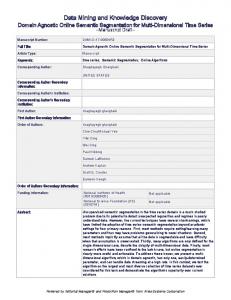
10.2 Spatial Data Mining and GIS Empowering a GIS with spatial data mining facilities presents some difficulties, since the design of a spatial data mining module depends on several aspects. The first aspect is the representation of spatial objects. In the literature, there are two types of data representations for the spatial data, that is, tessellation and vector [39]. They differ in storage, precision, and complexity of the spatial relation computation. The second aspect is the implicit definition of spatial relationships among objects. The three main types of spatial relationships are topological, distance, and directional relationships, for which several models have been proposed for the definition of their semantics (e.g., “9-intersection model” [14]). The third aspect is the heterogeneity of spatial objects. Spatial patterns often involve different types of objects (e.g., roads or rivers), which are described by completely different sets of features. The fourth aspect is the interaction between spatially close objects, which introduces different forms of spatial autocorrelation: spatial error (correlations across space in the error term), and spatial lag (the dependent variable in space i is affected by the independent variables in space i, as well as those, dependent or independent, in space j ). Classical data mining algorithms, such as those implemented in Weka [45], offer inadequate solutions with respect to these aspects. In fact, they work under the single table assumption [46], that is, units of analysis are represented as rows of a classical double-entry table (or database relation), where columns correspond to elementary (nominal, ordinal, or numeric) single-valued attributes. In any case, this representation neither deals with geographic data characterized by geometry, nor handles observations belonging to separate relations, nor naturally represents spatial relationships, nor takes them into account when mining patterns. Differently, geographic (or spatial) data are naturally modeled as a set of relations R1,...,Rn, such that each Ri has a number of elementary attributes and possibly a geometry attribute (in which case a relation is a layer). In this perspective, a (multi-)relational data mining approach seems the most suitable for spatial data mining tasks, since (multi)relational data mining tools can be applied directly to data distributed on several relations and since they discover relational patterns [13]. Example. To investigate the social effects of public transportation in a British city, a geographic data set composed of three relations is considered (see Figure 10.1). The first relation, ED, contains information on enumeration districts, which are the smallest areal units for which census data are published in the U.K. In particular, ED has two attributes, the identifier of an enumeration district and a geometry attribute (a closed polyline), which describes the area covered by the enumeration district. The second relation, BL, describes all the bus lines which cross the city. In this case, relevant attributes are the name of a bus line, the geometry attribute (a line) represents the route of a bus and the type of bus line (classified as main or secondary). The third relation, CE, contains some census data relevant for the problem, namely, the number of households with 0, 1, or “more than 1” cars. This relation also includes

C3974_C010.indd 261

11/17/08 7:13:43 PM

262

Geographic Data Mining and Knowledge Discovery ED

ID

Area

BL

03bsfc01

CE

ED 03bsfc01

Name

Line

Type

15a

Main

#households #households #households no car 1 car ≥2 cars 80

143

67

FIGURE 10.1 Representation of geographic data on the social effects of public transportation in a British city.

the identifier of the enumeration district, which is a foreign key for the table ED. A unit of analysis corresponds to an enumeration district (the target object), which is described in terms of the number of cars per household and crossing bus lines (bus lines are the task-relevant objects). The relationship between reference objects and task-relevant objects is established by means of a spatial join, which computes the intersection between the two layers ED and BL. Although several spatial data mining methods have already been designed by resorting to the multi-relational approach [4, 7, 21, 29, 30], most GISs which integrate data mining facilities [6, 16, 18] continue to frame the requests made by the spatial dimension within the classical data mining solution. Spatial properties and relationships of geographic objects are computed and stored as columns of a classical double-entry table, such that a classical data mining algorithm can be applied to the transformed data table. At present, only two of the GISs reported in the literature integrate spatial data mining algorithms designed according to the multi-relational approach. They are SPIN! [34] and INGENS [32]. SPIN! is the spatial data mining platform developed within the EU research project of the same name. SPIN! assumes an object-relational data representation and offers facilities for multi-relational sub-group discovery and multi-relational association rule discovery. Subgroup discovery [21] is approached by taking advantage of a tight integration of the data mining algorithm with the database environment. Spatial relationships and attributes are then dynamically derived by exploiting spatial DBMS extension facilities (e.g., packages, cartridges, or extenders) and used to guide the subgroup discovery. Association rule discovery [4] works in first-order logic and is only loosely integrated with a spatial database by means of some middle layer module that extracts spatial attributes and relationships independently of the mining step and represents these features in a first-order logic formalism. INGENS is our first attempt to empower a GIS with inductive learning capabilities. Indeed, it integrates the inductive learning system, ATRE, which can induce first-order logic descriptions of some concepts from a set of training examples. INGENS assumes an object-oriented representation of data organized in topographic maps. The geographic data collection is organized according to an object-oriented data model and is stored in the object store object oriented DBMS. Since object store does not provide automatic facilities for storing, indexing, and

C3974_C010.indd 262

11/17/08 7:13:43 PM

263


retrieving geographic objects, these facilities are completely managed by the GIS. In addition, INGENS integrates a Web-based GUI, where the user is simply asked to provide a set of (counter-) examples of geographic concepts of interest and a number of parameters that define the classification task more precisely. First-order descriptions learned by ATRE are only visualized in a textual format. The data mining process is condensed in a query written in SDMOQL [28], but the textual composition of the query is completely managed by the user.

10.3 INGENS 2.0 architecture and spatial data model The architecture of INGENS 2.0 is illustrated in Figure 10.2. It is designed as an open, highly extensible, Web-based architecture, where spatial data mining services are integrated within a GIS environment. The GIS functionalities are distributed among the following software components: • a Web-based GUI for supporting users in all activities, that is, user log-in and log-out, acquisition and editing of a topographic map, visualization and exploration of a topographic map, execution of a data mining request formulated by means of a spatial data mining query; • the User Management module for managing the access to the GIS (user creation, authentication, and history) for the different categories of users; • the Map Management module for managing requests of map creation, acquisition, update, delete, visualization, and exploration; • the Query Interpreter module for running user-composed SDMOQL queries and performing a spatial data mining task of classification or association rule discovery; • the Feature Extractor module for automatically generating conceptual descriptions (in first-order logic) of geographic objects, by making

?

?

SDMOQL Query Interpreter

FEATURE EXTRACTOR DATA MINING SERVER

MAP MANAGEMENT ? GUI

USER MANAGEMENT

Spatial DBMS

FIGURE 10.2 INGENS 2.0 software architecture.

C3974_C010.indd 263

11/17/08 7:13:43 PM

264


explicit (spatial) properties and relationships, which are implicit in the spatial dimension of data; • the Data Mining Server for running data mining algorithms; • the Spatial Database for storing both map data and information on the user history (logging user identifier and password, privileges, and spatial data mining queries executed in the past). The GUI can be accessed by four categories of users, namely, the GIS administrators, the map maintenance users, the data miners, and the casual end users. User profiles (e.g., authentication information, list of privileges) are stored in the database. The profile lists the topographic maps and the GIS functionalities to be accessed by the user. The administrator is the only user authorized to create, delete, or modify profiles of all other users of the GIS. The map maintenance user is in charge of upgrading the map repository stored in the spatial database by creating, updating, or deleting a map. The data miner can ask the GIS to discover either the operational definition of a geographic object or a spatial arrangement of geographic objects that are frequent on the topographic map under analysis. Finally, the casual end user is provided with geo-processing functionalities to navigate the topographic map, visualize geographic objects, belonging to one or more map layers (roads, parcels, and so on), and perform zooming operations. The user management module is in charge of the activities of creating, modifying, or deleting a user profile. Users are authorized to use only the GIS functionalities that match the privileges provided in their profiles. The map management module executes the requests of the map maintenance users. This component interfaces with the spatial database in order to create or drop an instance of a topographic map, as well as retrieve and display geographic objects belonging to one or more layers of a map. The query interpreter runs the SDMOQL queries composed by data miners. A query refers to one of the topographic maps accessible to the data miner and specifies the set of objects relevant to the task at hand, the kind of knowledge to be discovered (classification or association rules), the set of descriptors to be extracted from the map, the set of descriptors to be used for pattern description and optionally the background knowledge to be used in the discovery process, the geographic hierarchies, and the interestingness measures for pattern evaluation. The query interpreter’s responsibility is to ask the feature extractor to generate conceptual descriptions of the geographic objects extracted from the spatial database and then to invoke the inference engine of the data mining server. The conceptual descriptions are conjunctive formulae in a first-order logic language, involving both spatial and non-spatial descriptors specified in the query. SDMOQL queries are maintained in the user workspace and can be reconsidered in a new data mining process. Due to the complexity of the SDMOQL syntax, a user-friendly wizard is designed on the GUI side to graphically support data miners in formulating SDMOQL queries. The data mining server provides a suite of data mining systems that can be run concurrently by multiple users to discover previously unknown, useful patterns in geographic data. Currently, the data mining server provides data miners with two

C3974_C010.indd 264

11/17/08 7:13:44 PM

265


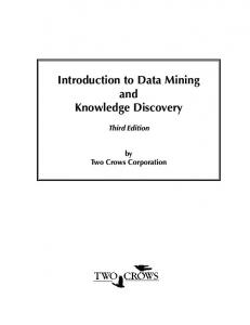
systems, ATRE [27] and SPADA [24]. ATRE is an inductive learning system that generates models of geographic objects from a set of training examples and counterexamples. SPADA is a spatial data mining system to discover multi-level spatial association rules, that is, association rules involving spatial objects at different granularity levels. In both cases, discovered patterns are returned to the GUI to be visualized and interpreted by data miners. The spatial database (SDB) can run on a separate computational unit, where topographic maps are stored according to an object-relational data model. The objectrelational DBMS used to store data is a commercial one (Oracle 10g) that includes spatial cartridges and extenders, so that full use is made of a well-developed, technologically mature spatial DBMS. Moreover, the object-relational technology facilitates the extension of the DBMS to accommodate management of geographic objects. At a conceptual level, the geographic information is modeled according to an object-based approach [41], which sees a topographic map as a surface littered with distinct, identifiable, and relevant objects that can be punctual, linear, or surfacic. Interactions between geographic objects are then described by means of topological, directional, and distance-based operators. In addition, geographic objects are organized in a three-level hierarchy expressing the semantics of geographic objects independently of their physical representation (see Figure 10.3). The entity object is a total generalization of eight distinct entities, namely, hydrography, orography, land administration, vegetation, administrative (or political) boundary, ground transportation network, construction, and built-up area. Each of these is in turn a generalization, for example, administrative boundary generalizes the entity’s city, province, county, or state. At a logical level, geographic information is represented according to a hybrid model, which combines both a tessellation and a vector model [39]. The tessellation

Object

Hydrography

Orography

Land administration

Parcel

River Font

Sea

Lake

Canal

Vegetation

Administration Construction Ground boundary transportation Built-up area

Park Cultivation Forest

City Province County State Contour slope

Slope

Level point

Road Ropeway Railway Bridge

Hamlet Town Main Regional Capital town capital

Building Airport Wall Power Boat Factory Deposit station station

FIGURE 10.3 Hierarchical representation of geographic objects at different levels of granularity.

C3974_C010.indd 265

11/17/08 7:13:44 PM

266

Geographic Data Mining and Knowledge Discovery MAP Id NUMBER Map MAP_TY

CELL Id NUMBER Mapld NUMBER Cell CELL_TY

GIF

LOGICAL_OBJECT Id NUMBER CellId NUMBER LogicalObject LOGICAL_OBJECT_TY

PHYSICAL_OBJECT Id NUMBER LogicalObjectID NUMBER GEOMETRY MDSYS.SDO_GEOMETRY

CellId NUMBER Gif STRING

FIGURE 10.4 Spatial data schema.

model partitions the space into a number of cells, each of which is associated with a value of a given attribute. No variation is assumed within a cell and values correspond to some aggregate function (e.g., average) computed on the original values in the cell. A grid of square cells is a special tessellation model called raster. In the vector model the geometry is represented by a vector of coordinates, which define points, lines, or polygons. Both data structures are used to represent geographic information in INGENS 2.0. The partitioning of a map into a grid of square cells simplifies the localization and indexing process. For each cell, the raster image in GIF format is stored, together with its coordinates and component geographic objects. These are represented by a vector of coordinates stored in the field Geometry of the database relation PHYSICAL OBJECT (see Figure 10.4), while their semantics are defined in the field LogicalObject of the database relation LOGICAL OBJECT. A foreign key constraint relates each tuple of PHYSICAL OBJECT to one tuple of LOGICAL OBJECT. Type inheritance is exploited to represent the conceptual hierarchy in Figure 10.3 at the logical level. Indeed, the type of the attribute LogicalObject (LOGICAL_OBJECT_TY) has eight subtypes, namely, HYDROGRAPHY_ TY, OROGRAPHY_TY, LAND_ADMINISTRATION_TY, VEGETATION_TY, ADMINISTRATIVE_BOUNDARY_TY, GROUND_TRANSPORTATION_TY, CONSTRUCTION_TY, and BUILDUP_AREA_TY. Each of these is in turn a generalization of new types according to the conceptual hierarchy. Spatial and non-spatial features can be extracted from geographic objects stored in the SDB. Feature extraction requires complex data transformation processes to make spatial properties and relationships explicit. This task is performed by the feature extractor module, which makes possible a loose coupling between data mining services and the SDB. The feature extractor module is implemented as an Oracle package of PL/SQL functions to be used in the spatial SQL queries.

C3974_C010.indd 266

11/17/08 7:13:44 PM

267


10.4 Spatial data mining process in INGENS 2.0 In INGENS 2.0 the spatial data mining process is activated and controlled by means of a query expressed in SDMOQL (see Figure 10.5). Initially, the query is syntactically and semantically validated. Then the feature extractor generates the conceptual representation of the geographic objects selected by the query. This representation, which is in a first-order logic language, is input to multi-relational data mining systems, which return spatial classification rules or association rules. Finally, the results of the mining process are presented to the user.

10.4.1 Conceptual Description Generation A set of descriptors used in INGENS 2.0 is reported in Table 10.1. They are either spatial or non-spatial. According to their nature, spatial descriptors can be classified as follows: 1. Geometrical, if they depend on the computation of some metric/distance. Their domain is typically numeric, for example, “extension.” 2. Topological, if they are invariant under the topological transformations (translation, rotation, and scaling). The type of their domain is nominal, for example, “region_to_region” and “point_to_region.” 3. Directional, if they concern orientation. The type of their domain can be either numerical or nominal, for example, “geographic direction.” 4. Locational, if they concern the location of objects. Locations are repre sented by numeric values that express coordinates. There are no examples of locational descriptors in Table 10.1. Some spatial descriptors are hybrid, in the sense that they merge properties of two or more of the above categories. For instance, the descriptor “line_to_line” that

VISUALIZATION QUERY OF SPATIAL DATA MINING

DATA MINING ENGINE FEATURE EXTRACTOR

DISCOVERED KNOWLEDGE

CONCEPTUAL DESCRIPTIONS

GDBMS

MAP REPOSITORY

FIGURE 10.5 Spatial data mining process in INGENS 2.0.

C3974_C010.indd 267

11/17/08 7:13:45 PM

268


Table 10.1 Set of Descriptors Extracted by the Feature Extractor Feature

Meaning

Value {true, false}

type_of(L) color(L) area(F) extension(F)

Cell C contains a logical object L Logical object L is composed of physical object F Type of L Color of L Area of F Extension of F

geographic_direction(F)

Geographic direction of F

{north-east, north-west, east, north}

line_shape(F) altitude(F)

Shape of the linear object F Altitude of F

{straight, curvilinear, cuspidal} [0.. MAX_ALT]

line_to_line(F1,F2)

Spatial relation between lines F1 and F2 Distance between lines F1 and F2 Spatial relation between regions F1 and F2 Spatial relation between a line F1 and a region F2 Spatial relation between a point F1 and a region F2

{almost parallel, al most perpendicular}

contain(C,L) part_of(L,F)

distance(F1,F2) region_to_region(F1,F2) line_to_region(F1,F2) point_to_region(F1, F2)

{true, false} 33 nominal values (e.g., river, road, ...) {blue, brown, black} [0..MAX_AREA] [0..MAX_EXT]

[0..MAX_DIST] {disjoint, contains, in side, equal, meet, covers, covered by, over lap} {along edge, intersect} {inside, outside, on boundary, vertex (i.e., F1 is a vertex of F2)}

expresses conditions of parallelism and perpendicularity is both topological (it is invariant with respect to translation, rotation, and scaling) and geometrical (it is based on the angle of incidence). In INGENS 2.0, geographic objects can also be described by two non-spatial descriptors, namely “type_of” and “color.” The former describes the type of a geographic object, according to the layer (street, parcel, river, and so on) it belongs to, while the latter describes the color (blue, black, or brown) used in the visualization of a geographic object. The descriptor “part_of” describes the structure of complex geographic objects, i.e., a geographic object can be formed by physical component objects, represented by separate geometries. There is no common mechanism to express the semantics of such different features. The semantics of topological relationships are based on the 9-intersection model [14], while the semantics of other features are based on mathematical methods of 2D-graphics [37] as described in [23]. Example (Geographic Direction). Let o be a geographic object associated with a line, that is,

C3974_C010.indd 268

o : {P1 = (x1, y1), …, Pn = (xn, yn)}.

11/17/08 7:13:45 PM


269

If a is the angle defined by the straight line L connecting P1 and Pn, that is:

α = arctg

x n − x1 , yn − y1

then the geographic direction of o is computed as follows: north

π π  π π  if α >  − ∨ α ≤ −  −  2 8 2 8

north east

π π  π if α ≤  − ∧ α > − 2 8 8

east northwest

if α ≤

π π ∧α > − 8 8

if α ≤ −

π π  π ∧ α > −  − . 2 8 8

This feature is computed only for geographic objects physically represented as lines.

10.4.2 Classification Rule Discovery Classification of geographic objects is a fundamental task in spatial data mining and GIS, where training data consist of multiple target geographic objects (reference objects), possibly spatially related with other non-target geographic objects (taskrelevant objects). The goal is to learn the concept associated with each class on the basis of the interaction of two or more spatially referenced objects or space-dependent attributes [22]. While a lot of research has been conducted on classification, only a few works deal with geographic classification. GISs empowered with classification facilities are reported in [6, 18]. These systems allow the learning of a classifier from data stored in a classical double-entry table (single-table assumption [46]). This is a severe restriction in GIS applications, where different geographical objects have different features (properties and relationships), which are properly modeled by as many data relations as the number of object types. To map the natural multi-relational form of geographic data into a single double-entry data table, GISs must integrate a transformation module that is in charge of computing the spatial features of geographic objects (e.g., a street crosses a river) and store them as columns of the double-entry table. This table can then be input to a wide range of robust and well-known classification methods which operate on a single table. This transformation (known as propositionalization) presents some drawbacks. In fact, the full equivalence between the original and the transformed training sets is possible only in special cases. However, even when possible, the output table size is unacceptable in practice [10] and some

C3974_C010.indd 269

11/17/08 7:13:45 PM

270


form of feature selection is required. Therefore, the transformed problem is different from the original one, for pragmatic reasons [7]. On the other hand, INGENS 2.0 overcomes the limitations of single table assumption by integrating a classification system, named ATRE [27], which resorts to a multi-relational data mining approach [13] to classify geographic objects. Indeed, a multi-relational approach to data mining (or MRDM) looks for patterns that involve multiple relations of a relational data representation. Thus, data taken as input by these approaches typically consist of several relations and not just a single one, as is the case in most existing data mining approaches. Patterns found by these approaches are called relational and are typically stated in a more expressive language than patterns defined in a single data table. Typically, subsets of first-order logic, which is also called predicate calculus or relational logic, are used to express relational patterns. In this way, the expressive power of predicate logic is exploited to represent both spatial relationships and background knowledge, thus providing functionalities to navigate relational structures of geographic data and generate potentially new forms of evidence, not readily available in flattened single double entry data table representation. The problem solved by ATRE is formalized as follows: Given • a set of concepts C1, C2, …, Cr to be learned; • a set of units of analysis (or observations) O described in a language LO; • a background knowledge BK described in a language LBK ; • a language of hypotheses LH that defines the space of hypotheses SH ; • a user’s preference criterion PC. Find a logical theory T ∈ SH , defining the concepts C1, C2,…, Cr, such that T is complete and consistent with respect to the set of observations and satisfies the preference criterion PC. The logical theory T is a set of first-order definite clauses [25], such as: cell(X1)=fluvial_landscape ← contain(X1,X2)=true, type_of(X2)=river, part_of(X2,X3)=true, line_to_line(X4,X3)=almost_parallel, part_of(X5,X4), type_of(X5)=street This clause can be interpreted easily as follows: If a cell X1 contains a river X2 with X2 represented by the line X3 and X3 almost parallel to the line X4 that represents a street X5, then the cell X1 can be classified as a “fluvial landscape.” This clause contains an operational definition of the fluvial landscape morphology. This definition can be used to recognize the unknown morphology for the cells of a new topographic map. The units of analysis are represented by means of a ground clause2 called objects. For example, if the units of analysis are the cells (reference objects) of a topographic map, then the body of an object describes the spatial arrangement of the geographic objects (task-relevant objects) within the cell, while the head may describe the landscape morphology (class) associated with the cell. The literal in the head of the clause is an example (either positive or negative) of the concepts C1, C2,…, Cr. 2

A ground clause contains no variables.

C3974_C010.indd 270

11/17/08 7:13:45 PM


271

FIGURE 10.6 Raster and vector representation (above) and symbolic description of a cell (below). The cell is an example of a territory where there is a fluvial landscape. The cell is extracted from a topographic chart (Canosa di Puglia 176 IV SW—Series M891) produced by the Italian Geographic Military Institute (IGMI) at scale 1:25,000 and stored in INGENS 2.0.

An instance of an object is reported in Figure 10.6, where the constant c8 denotes the whole cell, while the remaining constants (e.g., rv1_8, pc473_0, x20_8,…) denote the logical (river, street, parcel) or geometrical (line, point or polygon) component of the geographic objects in the cell. The descriptor cell(X) in the head denotes the known value of the morphology of the territory covered by the cell. The background knowledge BK can be defined in the form of first-order definite clauses, which allow the definition of new descriptors not explicitly encoded in a conceptual description of objects. An example of a clause that is part of a BK is the following: parcel_to_parcel(A,B)=C ←type_of(A)=parcel, type_of(B)=parcel, part_of(A,D)=true, part_of(B,E)=true, region_to_region(D,E)=C This clause allows the relationship C between two regions D and E to be automatically renamed as “parcel_to_parcel,” when D and E are parts of two parcels A and B. The completeness property of the output theory T holds when T explains all observations in O of the r concepts Ci, while the consistency property holds when T explains no counter-example in O of any concept Ci. The satisfaction of these properties guarantees the correctness of the induced theory with respect to O, but not necessarily with respect to new unseen observations. The selection of the clause in T is made on the grounds of an inductive bias [35], expressed in the form of preference criterion (PC). For example, clauses that explain a high number of positive examples and a low number of negative examples can be preferred to others. At the high-level, the learning strategy implemented in ATRE is sequential covering (or separate-and-conquer) [35], that is, one clause is learned (conquer stage), covered examples are removed (separate stage), and the process is iterated on the

C3974_C010.indd 271

11/17/08 7:13:46 PM

272


remaining examples. The conquer stage of this algorithm aims to generate a clause that covers a specific positive example, called seed. The most important novelty of the learning strategy implemented in ATRE is embedded in the design of the conquer stage. Indeed, the separate-and-conquer strategy is traditionally adopted by single concept learning systems that generate clauses with the same literal in the head at each step. In ATRE, clauses generated at each step may have different literals in their heads. In addition, the body of the clause generated at the i-th step may include all literals corresponding to those target concepts C1, C2,…, Cr for which at least a clause has been added to the partially learned theory in previous steps. In this way, dependencies between target concepts can be automatically discovered. An example of a logical theory, where the dependency between concepts “downtown” and “residential” is handled, is reported in the following: class(X)=downtown ← on_the_sea(X)=true, business_activity(X)=high. class(X)=residential ← contain(X,Y)=true, type_of(Y)=kindergarten, shopping_activity(X)=high. class(X)=residential ← close to(X,Y)=true, class(Y)=downtown, business_activity(X)=low. The order in which clauses of distinct target concepts have to be generated is not known in advance. This means that it is necessary to generate clauses with different literals in the head and then to pick one of them at the end of each step of the separate-and-conquer strategy. Since the generation of a clause depends on the chosen seed, several seeds have to be chosen, such that at least one seed per incomplete concept definition is kept. Therefore, the search space is actually a forest of as many search-trees (called specialization hierarchies) as the number of chosen seeds. A directed arc from a node (clause) C to a node C′ exists if C′ is obtained from C by adding a literal (single refinement step). The forest can be processed in parallel by as many concurrent tasks as the number of search-trees (hence, the name of separate-and-parallel-conquer for this search strategy). Each task traverses the specialization hierarchy top-down (or general-tospecific), but synchronizes traversal with the other tasks at each level. Initially, some clauses at depth one in the forest are examined concurrently. Each task is actually free to adopt its own search strategy, and to decide which clauses are worth testing. If none of the tested clauses is consistent, clauses at depth two are considered. The search proceeds toward deeper and deeper levels of the specialization hierarchies until at least a user-defined number of consistent clauses is found. Task synchronization is performed after all “relevant” clauses at the same depth have been examined. A supervisor task decides whether the search should carry on or not, on the basis of the results returned by the concurrent tasks. When the search is stopped, the supervisor selects the “best” consistent clause according to the user’s preference criterion. This separate-and-parallel-conquer search strategy provides us with a solution to the problem of interleaving the induction process for distinct concept definitions. It has the advantage that simpler consistent clauses are found first,

C3974_C010.indd 272

11/17/08 7:13:46 PM


273

independently of the predicates to be learned. Moreover, the synchronization allows tasks to save much computational effort when the distribution of consistent clauses in the levels of the different search-trees is uneven. A more detailed description of the search strategy implemented in ATRE and its optimization through caching techniques is reported in [5, 27].

10.4.3 Association Rule Discovery Association rules are a class of regularities introduced by Agrawal and Srikant [1], which can be expressed by an implication of the form:

A ⇒C(s, c),

where A(antecedent) and C(consequent) are sets of atoms, called items, with A ∩ B = f. s is called support and estimates the probability p(A ∪ C), while c is called confidence and estimates the probability p(C|A). A pattern P (s%) is frequent if s ≥ minsup. An association rule A ⇒ C (s%, c%) is strong if the pattern A ∪ C (s%) is frequent and c ≥ minconf. We call an association rule A ⇒ C spatial, if A ∪ C is a spatial pattern, that is, it expresses a spatial relationship among spatial objects. The problem of mining spatial association rules was originally tackled by Koperski [22], who implemented the module geo-associator of the spatial data mining system GeoMiner [18]. Similar to the classification task, the method implemented in geo-associator suffers from the limitations due to adapting the restrictive singletable data representation to the case geographic data. Weka-GPDM [6] is a further example of a GIS that includes facilities to discover spatial association rules. Once again, spatial features are extracted in a preprocessing step and stored as features of a single double-entry data table. Association rules are discovered in another step by applying the conventional association rule discovery algorithm included in Weka [45] to the single double-entry data table. Similar to the classification case, INGENS 2.0 overcomes limitations of single table assumption by integrating an association rule discovery system, named SPADA [24], which exploits the expressive power of a predicate logic to deal with spatial relationships in the original relational form. In addition, SPADA automatically supports a multiple-level analysis of geographic data. Indeed, geographic objects are organized in hierarchies of classes. By descending or ascending through a hierarchy, it is possible to view the same geographic object at different levels of abstraction (or granularity). Confident patterns are more likely to be discovered at low granularity levels. On the other hand, large support is more likely to exist at higher granularity levels. In general, the discovery of multi-level patterns (e.g., the most supported and confident) can be performed by forcing users to repeat independent experiments on different representations. In this way, results obtained for high granularity levels are not used at low granularity levels (or vice versa). Conversely, SPADA is able to explore altogether the search space at different granularity levels, such that patterns obtained for high granularity levels are used to control search at low granularity levels.

C3974_C010.indd 273

11/17/08 7:13:46 PM

274


The problem solved by SPADA is formalized as follows: Given • a set S of reference objects, which is the main subject of the analysis, • some sets Rk , 1 ≤ k ≤ m of task-relevant objects, • a background knowledge BK including spatial hierarchies Hk on objects in Rk , • M granularity levels in the descriptions (1 is the highest, while M is the lowest), • a set of granularity assignments ψk, which associate each object in Hk with a granularity level to deal with several hierarchies at once, • a couple of thresholds minsup[l] and minconf[l] for each granularity level l, • a language bias LB which constrains the search space. Find strong spatial association rules for each granularity level. The reference objects are the main subject of the description, while task-relevant objects are geographic objects that are relevant for the task at hand and are spatially related to the reference objects. For example, the cells may be the reference objects of our analysis, while the geographic objects within the cells are the task-relevant objects. In this case, properties and relationships of task relevant objects within each cell are computed by the feature extractor and stored as ground atoms, e.g., the spatial perpendicularity between the geographic objects g1 and g2 is represented by the ground atom almost_perpendicular(g1, g2). If g is a task-relevant object of the set Rk, then is_a(g, nj) establishes the association between a geographic object g and corresponding objects at the level j (j = 1, …, M) of the hierarchy Hk. Finally, for each cell c, the ground atom cell(c) identifies the unique reference object in the units of analysis. The task of spatial association rule discovery performed by SPADA is split into two sub-tasks: find frequent spatial patterns and generate highly confident spatial association rules. The discovery of frequent patterns is performed according to the levelwise method described in [33], that is, a breadth-first search in the lattice of patterns spanned by a generality order between patterns. In SPADA the generality order is based on q substitution [38]. The pattern space is searched one level at a time, starting from the most general patterns and iterating between candidate generation and evaluation phases. Once large patterns have been generated, it is possible to generate strong spatial association rules. For each pattern P, SPADA generates antecedents suitable for rules being derived from P. The consequent, corresponding to an antecedent, is simply obtained as the complement of atoms in P and not in the antecedent. Rule constraints are used to specify literals which should occur in the antecedent or consequent of discovered rules. In a more recent release of SPADA (3.1) [3], new pattern (rule) constraints have been introduced in order to specify exactly both the minimum and maximum number of occurrences for a literal in a pattern (antecedent or consequent of a rule). An additional rule constraint has been introduced to eventually specify the maximum number of literals to be included in the consequent of a rule. In this way, we are able to constrain the consequent of a rule requiring the presence of only the literal representing the class label and obtain useful patterns for classification purposes. Finally, the generation of patterns also takes into account a BK expressed in

C3974_C010.indd 274

11/17/08 7:13:46 PM


275

the form of first-order definite clauses. In this way, it is possible to simulate inferential mechanisms defined within a spatial reasoning theory. Moreover, by specifying both a BK and some suitable pattern constraints, it is possible to change the representation language used for spatial patterns, making it more abstract (human-comprehensible) and less tied to the physical representation of geographic objects. An example of a spatial pattern discovered by SPADA is the following: cell(A), contain(A,B), contain(A,C), is a(B,object), is_a(C,object), extension(C,[100..200.5]) (40%), which expresses a spatial containment relation between a cell A and some geographic objects B and C, where C is represented by a line with an extension between 100 and 200.5 m. This pattern occurs in 40% of the cells. The following spatial association rule: cell(A), contain(A,B), contain(A,C), is_a(B,object), is_a(C,object) ⇒ extension(C,[100..200.5]) (40%, 60%),

states that “in 60% of the cells (A), containing two geographic objects B and C, C is a line whose extension is between 100 and 200.5.” Since SPADA, like many other association rule mining algorithms, cannot process numerical data properly, these are discretized in equal-width intervals which are treated as ground terms. By taking into account hierarchies on task-relevant objects, we obtain descriptions at different granularity levels. For instance, by considering a portion of the logical hierarchy on geographic objects, in which both hydrography and administrative boundary are considered, specialization of objects is as follows: hydrography � administrative boundary �

object

A finer-grained spatial association rule can be the following: cell(A), contain(A,B), contain(A,C), is_a(B,administrativeBoundary), is_a(C,hydrography) ⇒ extension(C,[100..200.5]) (35%, 70%),

which provides better insight into the nature of the geographic objects B and C.

10.5 SDMOQL The syntax of SDMOQL is designed according to a set of data mining primitives designed to facilitate efficient, fruitful spatial data mining in INGENS 2.0. Seven primitives have been considered as guidelines for the design of SDMOQL. They are: 1. the set of geographic objects relevant to a data mining task, 2. the kind of knowledge to be discovered, 3. the set of descriptors to be extracted from a digital map (primitive descriptors),

C3974_C010.indd 275

11/17/08 7:13:46 PM

276


4. the set of descriptors to be used for pattern description (pattern descrip tors), 5. the background knowledge to be used in the discovery process, 6. the concept hierarchies, 7. the interestingness measures and thresholds for pattern evaluation. These primitives correspond directly to as many non-terminal symbols of the definition of an SDMOQL statement, according to an extended BNF grammar. Indeed, the SDMOQL top-level syntax is the following: ::= ; {;} ::= ¥ | | ::= mine analyze with descriptors [] {} [with ], where “[]” represents 0 or one occurrence and “{}” represents 0 or more occurrences, and words in bold type represent keywords. In Sections 10.5.1 to 10.5.5 the detailed syntax for each data mining primitive is both formally specified and explained through various examples of possible mining problems.

10.5.1 Data Specification The first step in defining a spatial data mining task is the specification of the geographic objects on which mining is to be performed. Geographic objects are selected by means of a query with a SELECT-FROM-WHERE structure, that is: ::= {UNION } ::= SELECT {, } FROM {, } [WHERE ] The SELECT clause should return a cell or objects of a layer (hydrography, orography, and so on), or logical objects of a specific type (river, street, and so on). Hence, the selected geographic objects must belong to the same symbolic level, namely, cell, layer, or logic object. More formally the FROM clause can contain either a group of cells, a set of layers, or a set of logic objects, but never a mixture of them. Whenever

C3974_C010.indd 276

11/17/08 7:13:46 PM


277

the generation of the descriptions of objects belonging to different symbolic levels is necessary, the user can obtain it by means of the UNION operator. The following are examples of valid data queries: Example (Cell-level query). The user selects cell 26 from the topographic map of Canosa (Apulia) and the feature extractor generates the description of all the geographic objects in this cell. SELECT x FROM x in Cell WHERE x->num_cell = 26 AND x->part map->map_name = “Canosa” Example 2 (Layer-level query). The user selects the orography layer from the topographic map of Canosa and the construction layer from any map. The feature extractor generates the description of the objects in these layers for all cells of the map of Canosa. SELECT x, y FROM x in Orography, y in Construction WHERE x->part_map->map_name = “Canosa” Example 3 (Logical object-level query). The user selects the objects of the logic type river, from cell 26 of the topographic map of Canosa. The feature extractor generates the description of the rivers in this cell. SELECT x FROM x in River WHERE x->part_map->map_name = “Canosa” AND x->log_incell->num_cell = 26

10.5.2 The Kind of Knowledge to be Mined The kind of knowledge to be discovered determines the data mining task in hand. Currently, SDMOQL supports the generation of either classification rules or association rules. The former are used for a predictive task, while the latter are used for a descriptive task. The top-level syntax is defined as follows: ::= | ::= classification as for {, } ::= association as key is The denotes the name to be associated to the set of (classification or association) patterns to be discovered in the data mining task formulated within the SDMOQL statement. In a classification task, the user may be interested in inducing a set of classification rules for a subset of the classes (or concepts) to which training examples belong. In this case, the subset of interest for the user is specified in the list.

C3974_C010.indd 277

11/17/08 7:13:46 PM

278


As pointed out, spatial association rules define spatial patterns involving both reference objects and task-relevant objects [4]. For instance, a user may be interested in describing a given area by finding associations between large towns (reference objects) and geographic objects in the road network, hydrography, and administrative boundary layers (task-relevant objects). The atom denoting the reference objects is called the key atom. The predicate name of the key atom is specified in the key is clause.

10.5.3 Specification of Primitive and Pattern Descriptors The analyze clause specifies which descriptors, among those automatically generated by the feature extractor, can be used to describe the geographic objects extracted by means of the first primitive. The syntax of the analyze clause is the following: analyze , where: ::= {, } parameters {, } ::= / ::= threshold . The specification of a set of parameters is required by the feature extractor to automatically generate some primitive descriptors. The language used to describe generated patterns is specified by means of the following clause: with descriptors where: ::= {; } ::= [cost ] | [with ] ::= {, } ::= | ::= constant [] ::= variable mode role ::= old | new | diff ::= ro | tro The specification of descriptors to be used in the high-level conceptual descriptions can be of two types: either the name of the descriptor and its relative cost, or the name of the descriptor and the full specification of its arguments. The former is appropriate for classification. The (classification or association) rules are expressed by means of descriptors specified in the with descriptors list. They are specified by Prolog programs on the basis of descriptors generated by the feature extractor. For instance, the descriptor “font_to_parcel/2” has two arguments which denote two logical objects, a font and a parcel. The topological relation between the two logical objects is defined by means of the clause:

C3974_C010.indd 278

11/17/08 7:13:46 PM


279

font_to_parcel(Font,Parcel) = TopographicRelation : type_of(Font) = font, part_of(Font,Point) = true, type_of(Parcel) = parcel, part_of(Parcel,Region) = true, point_to_region(Point,Region) = TopographicRelation. In association rule mining tasks, the specification of pattern descriptors corresponds to the specification of a collection of atoms: “predicateName(t1, …, tn),” where the name of the predicate corresponds to a , while describes each term ti, which can be either a constant or a variable. When the term is a variable, the mode and role clauses indicate, respectively, the type of variable to add to the atom and its role in a unification process. Three different modes are possible: old when the introduced variable can be unified with an existing variable in the pattern, new when it is not already present in the pattern, or diff when it is a new variable but its values must be different from the values of a similar variable in the same pattern. Furthermore, the variable can fill the role of reference object (ro) or task-relevant object (tro) in a discovered pattern during the unification process. The is key clause specifies the atom that has the key role during the discovery process. The first term of the key object must be a variable with mode new and role ro. The following is an example of specification of pattern descriptors defined by an SDMOQL statement: with descriptors contain/2 with variable mode old role ro, variable mode new role tro; type_of/2 with variable mode old role tro, constant; fluvial_landscape/1 with is key with variable mode new role ro; This specification helps to select only association rules where the descriptors fluvial_landscape/1, contain/2, and type_of/2 occur. The argument of “cell” is a new variable that plays the role of ro. The argument of the predicate “fluvial landscape” is always a new variable that plays the role of ro. The predicate “contain” links the ro with other geographic objects contained in the “fluvial_landscape.” Finally, the first argument of the predicate “type_of” is always an old variable, denoting a geographic object that plays the role of tro, whereas the second argument is a constant value that denotes the type of object (e.g., river, street, parcel). The following association rule: fluvial_landscape(X), contain(X,Y), type_of(Y,river), X≠Y ⇒ contain(X,Z), type_of(Z,font), X≠Z, Y≠X satisfies the constraints of the specification and expresses the co-presence of both a river and a font in a cell classified as a fluvial landscape.

10.5.4 Syntax for Background Knowledge and Concept Hierarchy Specification Many data mining algorithms use background knowledge or concept hierarchies to discover interesting patterns. Background knowledge is provided by a domain expert on the domain to be discovered. This can be useful in the discovery process.

C3974_C010.indd 279

11/17/08 7:13:46 PM

280


The SDMOQL syntax for background knowledge specification is the following: ::= [] {} ::= define knowledge {; } ::= use background knowledge of users {, } on {, } In INGENS 2.0, the user can define a background knowledge expressed as a set of definite clauses; alternatively, the user can specify a set of rules explicitly stored in a deductive database and possibly discovered in a previous step. An example of a background knowledge definition is reported in the following: Example (Definition of close_to). close_to(X,Y)=true :_region_to_region(X,Y)=meet. close_to(X,Y)=true :_close_to(Y,X)=true. while an example of the use of this background knowledge is reported in the following: Example (Import of close_to). use background knowledge of users UserName1 on close_to/2. Concept hierarchies allow knowledge mining at multiple abstraction levels [17]. In SDMOQL, a specific syntax is defined for the hierarchy: ::= [] [] ::= define hierarchy | define hierarchy for ::= use hierarchy of user . The following example shows how to define some hierarchies in SDMOQL: Example (Logical hierarchy on geographic objects). define hierarchy LogicalObject as level1: {Hydrography,Orography, ...} < level0: Object; level2: {River,Lake,See,Font,Canal...}