Geometric Integrability and Consistency of 3D Point Clouds

Geometric Integrability and Consistency of 3D Point Clouds George Kamberov Stevens Institute of Technology Hoboken, NJ 07030

Gerda Kamberova Hofstra University Hempstead , NY 11549

[email protected]

[email protected]

Abstract Numerous applications processing 3D point data will gain from the ability to estimate reliably normals and differential geometric properties. Normal estimates are notoriously noisy, the errors propagate and may lead to flawed, inaccurate, and inconsistent curvature estimates. FrankotChellappa introduced the use of integrability constraints in normal estimation. Their approach deals with graphs z = f (x, y). We present a newly discovered General Orientability Constraint (GOC) for 3D point clouds sampled from general surfaces, not just graphs. It provides a tool to quantify the confidence in the estimation of normals, topology, and geometry from a point cloud. Furthermore, similarly to the Frankot-Chellappa constraint, the GOC can be used directly to extract the topology and the geometry of the manifolds underlying 3D point clouds. As an illustration we describe an automatic Cloud-to-Geometry pipeline which exploits the GOC.

1. Introduction Presently it is possible to extract 3D point clouds from complex 3D scenes, often at real-time video rates. What is needed are automatic and computationally stable methods to extract geometry from noisy non uniform clouds. These methods must handle automatically under-sampled regions, for example, they have to deal with surface boundaries and resolve the ambiguities imposed by objects that are or appear to be tangent to each other. Furthermore, given the expected low quality of the data it is crucial to have methods to evaluate the consistency of the recovered geometry even in the absence of ground truth. We present a novel orientation integrability condition, the General Orientability Constraint (GOC), which will serve as a foundation to provide an approach to quantify the performance of geometry reconstruction techniques from 3D point clouds and meshes. Furthermore, the GOC can be used to enhance different reconstruction methods, e.g.,

[12, 17, 24, 28]. As an example, we use the integrability constraint to modify the automatic Cloud to Geometry Pipeline from [17]. This leads to a significant speed up in the geometry computation stage of the pipeline.

1.1. Related work Estimating normals and geometry There is a vast literature on geometry extraction from point clouds. It includes local polynomial fits, global smooth approximations, Voronoi/Delaunay-based methods, and level set methods, for example, [1, 2, 7, 11, 25, 30]. Earlier heuristic approaches gave no guarantees, but new powerful methods do give guarantees of faithfulness to the underlying continuous shape in the limit of infinitely dense data [5, 6]—under somewhat restrictive assumptions on object smoothness and the evenness of the sampling. The estimation of the normals is a key step in geometry reconstruction – it is also notoriously prone to errors. These errors propagate and lead to unreliable estimates of local differential geometric properties. There are other factors contributing to the errors in the geometry estimates, e.g., discretization. As a result, many authors consider local differential geometric estimates unreliable [8, 9]. A number of authors have studied the reliability of orientation estimates. Dey et al. [4] have performed empirical comparisons of several approaches given ground truth data. Theoretical error bounds for a number of methods are derived in [22, 23]. The bounds derived by Mitra et al. [23] are only for the method for estimating normals presented in [23] (thus it works well if the data is properly sampled and one has sensor noise model, but the method heuristics fail on data sets like the one in Figure 2). [22] deals with surfaces of the form z = f (x, y).

Integrability constraints for normals on graphs Frankot and Chellappa [10] popularized the integrability condition that must be satisfied by a vector field (N1 (x, y), N2 (x, y), N3 (x, y)) to be the orientation

To Appear in Proc. ICCV 2007, Rio DeJaneiro, Oct 14-20, 2007.

and

(normal vector field) to a graph z = f (x, y), ∂ N1 ∂ N2 = . ∂y N3 ∂x N3

(1)

Many authors have used integrability on graph surfaces to help reconstruction and resolve ambiguities, for example, [9, 10, 27]. Using the conformal geometry approach to surface theory from [18] we look for integrability constraints satisfied by the orientation of a smooth surface in R3 , not necessarily a graph. 1.1.1 Conformal geometry of surfaces in R3 : background Conformal surface immersions provide a convenient machine to treat general surfaces in R3 , including surfaces with self-intersections. Following [16, 18] we think of a smooth surface, S ⊂ R3 , as a vector-valued map, f , from some orientable two-dimensional manifold M 2 into Euclidean three space such that S = f (M 2 ), the map f is an immersion with Gauss map N. The Gauss map assigns to each point on M 2 a unit vector orthogonal to S. The GOC and the computations underlying the framework in [16] are based on analysis of the differentials df and dN of the immersion and the Gauss map. A differential of a map is just a one-form whose inputs are tangent vectors and whose outputs are the corresponding directional derivatives. Recall that the vector-valued map f : M 2 → R3 is an immersion if and only if its differential has trivial kernel, that is, df (v) 6= 0 if v 6= 0. The immersion and the Gauss map induce a complex structure J on M 2 defined as follows: let v be a vector tangent to M 2 , then J(v) is the unique tangent vector satisfying df (J(v)) = N × df (v) .

ω(v) :=

1 (dN(v) − N × dN(J(v))) 2 dN(v) − τ (v).

where K is the Gauss curvature (of f ). Furthermore the principal curvature directions are expressed in closed form formulae involving df (v) and the dot products ω(v) · df (v) and ω(v) · df (J(v)).

2. GOC: The General Orientability Constraint 2.1. Smooth surfaces Similarly to the Frankot-Chellappa we will search for the differential equations satisfied by the Gauss map N for the integrability constraint. In fact the constraint involves the form τ and it follows from the identity (5) and its derivatives. To express the constraint as partial differential equations we will use isothermal coordinate systems (x, y) with respect to f (i.e., conformal parameters with respect to the complex structure J). A coordinate system (x, y) is isothermal with respect to f iff: ∂f ∂f =N× . ∂y ∂x

(8)

Such coordinate systems are defined in a neighborhood of every point. The condition of being conformal parameters can be expressed in terms of the complex structure as µ ¶ ∂ ∂ =J . (9) ∂y ∂x Denote by τ x and τ y the components of τ with respect to the conformal parameters (x, y) so τ = τ x dx + τ y dy, where τx

=

τy

=

µ 1 ∂N −N× 2 ∂x µ 1 ∂N +N× 2 ∂y

(10) ¶ ∂N ∂y ¶ ∂N ∂x

(11) (12)

(3)

Notice that in regions where the mean curvature is identically zero (5) leads to the constraint

(4)

τ =0

The fundamental identity

(13)

or equivalently

− Hdf = τ,

(5)

where H is the mean curvature function implies that for every nonzero tangent vector v we have H=−

(ω(v) · df (v))2 ((ω(v) · df (J(v))2 − , (7) |df (v)|4 |df (v)|4

(2)

Here × denotes the cross-product in R3 . Essentially J is a counter-clockwise rotation in the tangent plane by 90o . The key to the conformal method for computing differential geometric properties [14] and to the orientability constraint is to look at two R3 -valued 1-forms τ and ω defined in [18] by τ (v) :=

K = H2 −

τ (v) · df (v) |df (v)|2

(6)

∂N ∂N =N× . (14) ∂x ∂y In regions where the mean curvature is not identically zero we must differentiate (5) to obtain the constraint. By comparing the coefficients of dτ = dH ∧ d f ,


(15)

where ∧ denotes the usual edge product of 1-forms, we obtain the constraint ∂δx ∂δy =− , ∂y ∂x

(16)

where δx and δy are uniquely defined by dτ = (δx τx + δy τy ) dx ∧ dy.

(17)

Equation (16) is a third order partial differential equation for the components of N. Thus we can summarize the GOC: Theorem 1 If N is the orientation of a C 4 conformal immersion in R3 of a surface equipped with a complex structure J, then in a neighborhood of every point, N satisfies either (14) or (16). Here (x, y) are conformal with respect to J. Remark The GOC does encompass the FrankotChellappa conditions, but one has to do a change of variables first. It is easy to see that in general the (x, y) parameters used to parameterize a graph f (x, y) = (x, y, z(x, y)) are not isothermal.

2.2. Discrete GOC on 3D point clouds We propose an approach to address orientation integrability of discrete oriented, topologized clouds in R3 without requiring such high order smoothness of the underlying surfaces as in Theorem 1. Definition 1 An oriented point cloud in R3 is a set © ª 3 (p, N) ∈ R × S 2 of 3D points with a ”normal” vector attached to each point; the 3D points form the underlying point cloud. The cloud is topologized if it is equipped with a connectivity graph which specifies the neighbors of each point. Integrability constraints are expressed in terms of derivatives or path integrals. Thus we will measure integrability in the context of a chosen discrete calculus approach. Discrete GOC assumptions: Assume that we are given a topologized oriented point cloud and that a method for computing first order directional derivatives ( along tangent vectors) has been selected. So for every tangent vector u we can estimate the directional derivatives dN(u) and df (u) from the oriented point cloud. The derivatives estimates are tangent-valued, i.e., orthogonal to N (in agreement with differential geometry). There are many approaches to building a topologized oriented point cloud from a cloud of 3D points, e.g., one could use one of the many polyhedral reconstruction methods discussed earlier, or say the methods in [13, 15, 20, 21, 23]. For

a given topologized oriented cloud, one can select among many possible discrete difference schemes to compute directional derivatives. In Section 3 we apply the proposed approach to GOC for a particular orientation-topologydiscrete calculus scheme. To derive the GOC we look at the fundamental identity (5). It implies that in integrable case when the normals are properly chosen and there is no noise due to discretization: τ (v) × df (v) = 0, for every tanget vector v

(18)

and h(v) :=

τ (v) · df (v) is independent on v |df (v)|2

(19)

Thus, the extent to which integrability is violated is measured by the rate of failure of (18) and (19). At each point P = (p, N) in the oriented cloud we define the penalty terms I α(P ) = | sin (] (τ (v), df (v))) |dv (20) A(P )

and χ(P ) = Var(h(v) | v ∈ A(P )),

(21)

here A(P ) is the set of unit tangent vectors based at p in which we can compute cross products τ (v) × df (v) and the dot products h(v), (19). In this paper we use A(P ) to be the set of unit vectors in direction of the tangential projections → of the vectors pqi where (qi , Ni ) are the neighbors of P . So the integral (20) is just a finite sum over all neighbors of the point. We measure the orientation integrability of an oriented point cloud C = {P = (p, N)} by X O(C) = (α(P ) + χ(P )). (22) P ∈C

3. The Cloud to Geometry Pipeline C2G Using O(C) we modified the automatic pipeline introduced in [17].

3.1. Topology and Calculus To define a topology on a oriented point cloud we use the proximity likelihood introduced in [15] and follow the framework in [16]. Given a choice of geometric scale ρ, the proximity likelihood 0 ≤ ∆P (Q) ≤ 1 defined in [15] measures the likelihood that the oriented point Q is a neighbor of the oriented point P on a surface patch. The likelihood incorporates three estimators of surface distance: a linear estimator based on Euclidean distance, a quadratic estimator based on the cosine between normals, and a third order estimator δP which is crucial in distinguishing points which are far on the surface but close in Euclidean distance


(δP (Q) = O(s3 ) where s is the surface distance between the points). Thus, neighborhoods built using the proximity likelihood based on ∆P (Q) are in general tighter than the usual approach using k-nearest Euclidean neighbors. We use the proximity likelihood to build neighborhoods around each oriented point P that have the smallest possible radius in terms of surface distance (for the given scale choice) and the smallest number of neighbors that still provide all the available information about the normal distribution around P . We call these neighborhoods ∆-neighborhoods. The ∆-neighborhoods provide a tool to classify the points of an oriented cloud as isolated points, curve points, boundary surface points, or interior surface points [16]. Isolated, curve and surface boundary points are called cloud boundary points. A surface point is distinguished by the property that one can use the ∆ neighborhood to compute the orientation in at least two orthogonal directions tangential directions at the point, i.e., two orthogonal directions emanating from the point and perpendicular to the normal at the point. The point is an interior surface point if one can use the ∆-neighborhood to compute the orientation in a full circle of tangential directions, otherwise the surface point is a surface boundary point. The surface points are samples of 2D manifolds and we can compute surface differential properties following the conformal method [14]. Finding a ∆-neighborhood of a point is a pretty straightforward region growing procedure. The neighbors of a point are determined by starting at the point and following the gradient of the proximity likelihood inside the voxel determined by the geometry scale. The process stops if the point is identified as an interior surface point or upon exiting the voxel. In the later case the point is automatically classified as a cloud boundary point. With this approach there is no extra cost to treat automatically scenes with multiple objects and surfaces with boundary. To define directional derivatives we identify surface immersions with their images so the tangent vectors are actually vectors in R3 , i.e., a tangent vector v at a oriented point (p, N) is just a 3D vector perpendicular to N and J(v) = N × v. Each directional derivative df (v) is just v. A unit tangent vector v at P = (p, N) is called radial at P if it is parallel with the tangent projection of an edge from a point to one of its ∆- neighbors in the cloud. If v is a radial vector, then the directional derivative dN(v) is computed by a first order difference along the edge from P to its neighbor and dN(J(v)) is computed by a linear interpolation of the directional derivatives along the radial directions closest to J(v). This setup enables us to compute the penalty terms α(P ) (see (20)) and χ(P ) (see (21)) and therefore the integrability deviation measure O(C) of the topologized oriented point cloud (see (22) ).

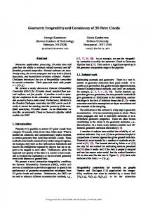
Figure 1. The C2G pipeline.

3.2. The Pipeline Outline The stages and the data flow in the Cloud-to-Geometry (C2G) pipeline are laid out in Figure 1. The pipeline is based on the ideas introduced in [17]. The pipeline takes as input a 3D point cloud and outputs: 1. A point-based reconstruction of the scene geometry: each point is equipped with a normal and a neighborhood of points closest to it in terms of surface distance; the points are classified as isolated, curve, and surface points, and the surface points are divided into interior and boundary points; the connected components of the topologized cloud are identified thus segmenting the scene into geometric objects represented by 0D, 1D, and 2D submanifolds. 2. Estimates of differential geometric properties (curvatures and principal curvature directions) at each surface point. The path from 3D point samples to a complete description of scene geometry leads through several stages. The 3D point cloud is a sample of the underlying scene with noise arising from sensor errors or uncertainty in the environment. In the first stage we use a clustering method of [29] to group these noisy samples into local primitives which incorporate localized scene measurements plus uncertainties. The scale at which this is done, we call the clustering/localization scale. The primitives are fish scales [29] and consist of a local covariance ellipsoid approximating the 3D spatial density, with the smallest eccentricity direction encoding the (unoriented) surface normal line. The clustering scales are established automatically and adaptively [3]. The next stage uses the unorganized fish-scales to establish orientation and surface topology (i.e., connectivity), followed by the geometry. The key parameter is the geometry/voxelization scale—the scale at which local shape “texture” can be distinguished. Here we will assume that the geometry details scale is chosen. We have developed methods to learn this scale as we build the orientation and topology, but will discuss them in a separate paper due to lack


of space and to keep the discussion focussed. To compute orientation and topology, we follow [16, 17]. This approach gives rapid orientation of the cloud starting from local estimates of the unoriented surface normals. A prime advantage is that, unlike previous methods based on triangulations and parameterizations, our method does not commit prematurely to assignments of surface patch orientation based on local information. The topology is computed by finding the ∆neighborhood of each oriented point, then the orientation is iteratively re-evaluated by comparing orientations and possibly flipping the orientations of adjacent connected components. The process continues while the integrability deviation measure O(C) continues to decrease. Note Thus, the topology-orientation stage minimizes the integrability deviation measure. The orientation-topology iteration is designed to analyze automatically the ambiguities occurring in regions where different surfaces meet [17]. The hardest case—tangent surfaces—is handled by analyzing the proximity likelihood distributions in the different candidate neighborhoods (coming from different bifurcation branches). This approach allows us to resolve automatically cases (See Figures 2 and 3) where polygonal-based approaches and competing pointbased approaches (e.g., [23]) need human intervention. To compute the surface differential properties estimates we modify the conformal method technique [19, 14]. We use the formulae (6), (7), and the closed form expressions for the principal curvature directions. Instead of computing redundant estimates along all possible radial directions as in [19, 14] and then averaging, we use the estimates along the radial direction v for which the penalty | sin (] (τ (v), df (v))) | is minimal. Thus C2G needs a single pass through all neighbors of a point instead of the three passes needed in [17]. As a result C2G, is considerably faster than the reference pipeline [17]. Note Essentially we replace average estimates with most likely estimates, as measured using the GOC.

Figure 3. (Left) A cloud 3D point cloud obtained from stereo [3]; (Middle and Right) the two largest 2D components extracted from the 3D point cloud. The quality of the cloud segmentation into manifolds matches the one reported in [17].

4. Summary We presented an orientation integrability constraint applicable to general 3D clouds. It provides a method to optimize the reconstruction of topology and orientation from a 3D point cloud. The orientation integrability constraint and the underlying approach to estimating the consistency of the topology, orientation, and geometry reconstructions provide methods to speed up and improve the reliability of the the computation of differential geometric properties by taking the most likely estimates. The proposed approach is implemented in a pipeline that deals successfully with clouds in which previous methods fail, and provides geometric quality of the geometry estimates comparable to the original conformal method.

References [1] M. Alexa, J. Behr, D. Cohen-Or, S. Fleishman, D. Levin, C. T. Silva, ”Computing and Rendering Point Set Surfaces”, Trans. Vis. Comp. Graph., Volume 9(1): 3-15, 2003. 1 [2] N. Amenta and Kill, Y. J., ”Defining Point-Set Surfaces”, ACM Trans. on Graphics, vol. 23(3), 264-270, Special Issue: Proceedings of SIGGRAPH 2004. 1 ´ [3] H. Cornelius, Sara, R., Martinec, D., Pajdla, T., Chum, O., Matas, J., ”Towards Complete Free-Form Reconstruction of Complex 3D Scenes from an Unordered Set of Uncalibrated Images,” SMVP/ECCV 2004, vol. LNCS 3247, pp. 1-12, Prague, Czech Republic, May 2004. ACM, pp. 280-289, 2004. 4, 5 [4] T. K. Dey, Li, G., Sun, J., ”Normal Estimation for Point Clouds: A Comparison for a Voronoi Based Method”, Eurographics Symposium on Point-Based Graphics (2005), M. Pauly, M. Zwicker, (Editors). 1 [5] T. K. Dey, Sun, J., ”An Adaptive MLS Surface for Reconstruction with Guarantees” , Tech. Rep. OSU-CISRC-4-05TR26, Apr. 2005. 1

Figure 2. Two tangent surfaces: (Left) The original point cloud sampled from a sphere touching a plane. (Right) The two largest connected components extracted by the C2G pipeline: part of the sphere and part of the plane.

[6]

T. K. Dey, Sun, J., ”Extremal Surface Based Projections Converge and Reconstruct with Isotopy”, Tech. Rep. OSUCISRC-05-TR25, Apr. 2005. 1

[7]

H. Edelsbrunner, Mucke, E.P., ”Three-dimensional alpha shapes,” ACM Trans. Graph., Volume 13(10, 43-72, 1994. 1


[8] Flynn, P.J., and Jain, A.K. On Reliable Curvature Estimation, Proc. IEEE Conf. Comp. Vis. Patt. Rec., pp 110-116, 1989. 1 [9] D.A. Forsyth, “Shape from texture and integrability,” Proc. ICCV01, pp 447–452, 2001. 1, 2 [10] R. T. Frankot and Chellappa, R., “A Method for Enforcing Integrability in Shape from Shading Algorithms”, IEEE Transactions on Pattern Analysis And Machine Intelligence, vol 10(4), 439–451, July 1988. (See also Horn and Brook, Shape from Shading, MIT Press, 1989.) 1, 2 [11] M. Gopi, Krishnan, S., Silva, C. T., ”Surface reconstruction based on lower dimensional localized Delaunay triangulation”, EUROGRAPHICS 2000, Computer Graphics Forum, vol 19(3), 2000. 1 [12] C. Grimm,”Parameterization using Manifolds,” International Journal of Shape Modeling, 10(1): 51-80, 2004. 1 [13] H. Hoppe, DeRose, T., Duchamp, T., McDonald, J., Stuetzle, W. ”Surface reconstruction from unorganized points”, Comp. Graph. (SIGGRAPH ’92 Proceedings), 26, 71–78, (1992) 3 [14] G. Kamberov, G. Kamberova, ”Conformal Method for Quantitative Shape Extraction: Performance Evaluation”, ICPR 2004, Cambridge, UK, August, 2004, IEEE Proceedings Series, 2004 2, 4, 5 [15] G. Kamberov, G. Kamberova,”Topology and Geometry of Unorganized Point Clouds”, 2nd Intl. Symp. 3D Data processing, Visualization and Transmission, Thessaloniki, Greece, IEEE Proc. Series, in cooperation with Eurographics and ACM SIGGRAPH, 2004. 3 [16] G. Kamberov, Kamberova, G., Jain, G., ”3D shape from unorganized 3D point clouds”, Intl. Symposium on Visual Computing, Lake Tahoe, NV, Springer Lecture Notes in Computer Science, 2005. 2, 3, 4, 5

[22] D. Meek, Walton, D., ”On surface normal and Gaussian curvature approximations given data sampled from a smooth surface.” Computer-Aided Geometric Design, 12:521-543, 2000. 1 [23] N. Mitra, N. Nguyen, and L. Guibas ”Estimating surface normals in noisy point cloud data,” International Journal of Computational Geometry & Applications, Vol. 14, Nos. 4&5, 2004, pp. 261–276. 1, 3, 5 [24] D. Nehab, Rusinkiewicz, S., Davis, J., and Ramamoorthi, R., “Efficiently Combining Positions and Normals for Precise 3D Geometry”, ACM Transactions on Graphics (Proc. SIGGRAPH). 24(3) August 2005. 1 [25] M. Bertalmo, Li-Tien Cheng, Osher, S., Sapiro, G., ”Variational problems and partial differential equations on implicit surfaces”, Volume 174 , Issue 2, 2001. 1 [26] S. Park, Guo, X., Shin, H.., and Qin, H., ”Shape and appearance repair for incomplete point surfaces,” Proc. ICCV 2005. [27] N. Petrovic, I. Cohen, B. Frey, R. Koetter, and T. Huang. “Enforcing integrability for surface reconstruction algorithms using belief propagation in graphical models”. In Proc. Conf. Computer Vision and Pattern Recognition (CVPR01), 2001. 2 [28] M. Pollefeys et al. Image-based 3d recording for archaeological field work. CG&A, 23(3):20–27, May/June 2003. 1 ˇ ara and Bajcsy, R., ”Fish-Scales: Representing Fuzzy [29] R. S´ Manifolds”, Proc. Int. Conference on Computer Vision, Bombay, India, Narosa Publishing House, 1998. 4 [30] H. Xie, McDonnell, K. , and Qin, H., Surface reconstruction of noisy and defective data sets, Proc. Visualization 04, pp. 259-266, 2004. 1

[17] G. Kamberov, Kamberova, G., Chum, O., Obdrzalek, S., ˇ Martinec, D., Kostkova, J., Pajdla, T., Matas, J., and Sara, R., ” 3D Geometry from Uncalibrated Images,” Proc. 2nd Intl. Symposium on Visual Computing, Lake Tahoe, NV, Springer Lecture Notes in Computer Science, Vol. 4292 II: 802–813, 2006. 1, 3, 4, 5 [18] G. Kamberov, P. Norman, F. Pedit, U. Pinkall, ”Quaternions, Spinors, and Surfaces”, American Mathematical Society , 2002, ISBN 0821819283. 2 [19] G. Kamberov, Kamberova, G., ”Shape Invariants and Principal Directions from 3D Points and Normals”, Proceedings of 10th Intl. Conf. in Central Europe on Computer Graphics and Visualization, 2002, Plzen. Journal of WSCG, Volume 10, pp 537-544, 2002. 5 [20] J. Klein, Zachmann, G., ”Point cloud surfaces using geometric proximity graphs”, Computers & Graphics, 28 (2004) 839-850. 3 [21] J. Lalonde, R. Unnikrishnan, N. Vandapel, and M. Hebert ”Fifth Scale Selection for Classification of Point-sampled 3D Surfaces,” Proc. International Conference on 3-D Digital Imaging and Modeling (3DIM 2005), 2005. 3
