GEOMETRIC SENSITIVITY OF THREE-DIMENSIONAL SEPARATED FLOWS
Erica M. Cherry Mechanical Engineering Department Stanford University Stanford, CA 94305, USA
[email protected]
Christopher J. Elkins Mechanical Engineering Department Stanford University Stanford, CA 94305, USA
[email protected]
John K. Eaton Mechanical Engineering Department Stanford University Stanford, CA 94305, USA
[email protected]
ABSTRACT Experiments were performed to determine the mean velocity field in two three-dimensional diffusers with the same fully-developed channel inlet but slightly different expansion geometries. Magnetic Resonance Velocimetry was used to collect velocity data. Both diffuser flows exhibited three-dimensional boundary layer separation but the size and shape of the separation bubble exhibited a high degree of geometric sensitivity dependent on the dimensions of the diffuser. Background Computational fluid dynamics (CFD) has evolved to the point where flow simulation plays a major role in the design of many high Reynolds number systems. This is particularly true for devices where pressure gradients are favorable, resulting in thin boundary layers and generally accurate predictions. However, the situation is different for flows containing regions of strong adverse pressure gradient where rapid boundary layer growth, flow separation, and associated unsteadiness can play an important role in determining overall device performance. In such flows, even the most advanced CFD codes are not reliable enough to make design decisions without corroborating experimental data. For example, a recent collaborative effort (Mellen et al., 2003) compared large eddy simulation results from multiple groups to a 2D airfoil experiment with mild trailing edge separation. There was considerable variation between the predictions of different codes, and no one method showed consistently good agreement with experimental data in the separated flow region. Turbulence modeling continues to be a major issue in separated flow prediction, probably because the mean flow characteristics change very rapidly from attached boundary layer, to incipient separation with an inflectional boundary layer profile, to a fully separated flow, and possibly through reattachment. As a result, the turbulence has highly non-equilibrium characteristics that are difficult to predict, even when the models do not assume equilibrium structure. Song & Eaton (2004) examined the Reynolds number scaling of a simple 2D separated flow with smoothwall separation from a curved ramp. They identified five
different regions in the flow that each had its own scaling behavior. While there are continuing efforts to find universal models (c.f. Leschziner, 2005), it is likely that carefully calibrated models for specific classes of separated flows will be required for some time to come. We believe that significant advances in separated flow prediction can only be achieved by careful comparison of CFD calculations with a range of separated flow data. The range of validity of various turbulence models and numerical implementations must be established, before they can be used for design purposes. A critical point in considering test cases is that almost all practical separated flows are three dimensional, even in the mean. Model developers and experimenters both prefer 2D flows because of the savings in computational resources and experimental effort. However, even nominally 2D flows may be strongly affected by three dimensionality. For example, the widely used 10 degree plane diffuser studied by Obi et al. (1993) and later by Buice and Eaton (2000) required an extremely high aspect ratio and complex endwall separation control systems to force the flow to be 2D. One must question if the calculations and experiments can be compared without accounting for this separation control. A further issue with many previous experiments in separated flows is that the boundary conditions are not fully defined or are difficult to exactly mimic in simulation. The seminal separation bubble study done by Simpson and co-workers (c.f. Simpson, 1981) had a complex opposite wall including multiple suction and blowing slots to insure 2D separation on a flat wall. The European collaborative airfoil experiment described in Mellen et al. (2003) used the same airfoil model in two different large wind tunnels and found different drag coefficients, probably due to windtunnel interference effects. The experiment of Song and Eaton (2004) used a curved ramp installed on the bottom wall of a wind tunnel leaving open the question of the appropriate outer-layer boundary condition. Separation behavior may be very sensitive to small changes in boundary conditions, so it is not possible to fully test a turbulence model if discrepancies between experiment and computation may be caused by incorrect or imprecise boundary condition prescription.
The overall goal of the present research is to develop 3D separated flow test cases that can be directly compared to CFD computations. In our opinion, such experiments should be conducted in fully 3D geometries allowing specification of simple boundary conditions (noslip and impermeability) on all bounding surfaces. The widespread availability of parallel computers and new three-dimensional measurement techniques means that it is now practical to conduct both the experiments and computations on the full 3D geometry. Furthermore, following the lead of Obi et al. (1993), Buice and Eaton (2000), and Gullman-Strand et al. (2004) we chose to use fully developed channel-flow inlet conditions. Thus, it is relatively simple for a modeler to obtain inlet conditions at any level of fidelity using well-qualified simulation techniques for fully-developed flows. In line with these goals, we have conducted experiments on two geometrically-simple, threedimensional diffusers with fully developed channel inlets. Diffuser flows have been used to study separated flows for many years, although in most cases the flows have been nominally two-dimensional. Ashjaee and Johnston (1980) collected detailed velocity, pressure, and separation location data for symmetric, 2D, straight-walled diffusers of opening angles between 8 and 24 degrees. For high angle diffusers, they found stall switch in which the separated region would move back and forth between the two diverging walls, often with a period measured in hours. The experiment was symmetric within manufacturing tolerances, and it was impossible to predict where the stall would develop initially. Clearly this phenomenon is more relevant to idealized experiments than practical applications. In the present experiments, we specifically avoided any symmetries to eliminate this problem. Recently, three 2D diffuser experiments have been widely used for comparison to CFD predictions. Obi et al (1993) examined an asymmetric diffuser with an expansion ratio of 4.7 and an expansion angle of 10 degrees. This flow geometry was simulated using LES techniques by Kaltenbach et al (1999). They noted that the Obi et al. data did not satisfy 2D mass conservation-the mean velocity profiles on the centerline indicated a 15% gain in mass flow rate near reattachment. This suggested the presence of strong mean-flow three dimensionality. Buice & Eaton (2000) attempted to replicate the Obi et al. experiment with an even larger aspect ratio (40:1). They found strongly 3D flow with the separation bubble growing from one end wall of the diffuser instead of from the diverging wall. This three dimensional separation was controlled using both suction and splitter plates on the end walls. Gullman-Strand et al. (2004) used a similar high aspect ratio apparatus to examine an asymmetric 8.5 degree diffuser. They used endwall suction to control three dimensionality and crossstream LDA measurements to show that the flow near the centerplane was 2D. The experiment included detailed turbulence data allowing direct comparison to some of the terms modeled in CFD calculations. The specific goals of the present experiment are to provide highly detailed three component mean velocity data in a simple, but fully three-dimensional diffuser. Magnetic resonance velocimetry (Elkins et al., 2003) is used to provide three-component velocity data throughout the flow field. In order to investigate the sensitivity of the separated flow to relatively small geometric changes, diffusers with two slightly different geometries are examined.
Experiment The working fluid for all of the experiments was water. Gadolinium-based contrast agent (Omniscan, Nycomed, Inc.) was added to the water in a concentration of 0.5%. A schematic of the recirculating flow loop is shown in Figure 1. A centrifugal pump (Little Giant model no. TE-6MD-HC) circulated water at a flow rate of 20.3 L/min. The average volume flow rate was measured using a Signet Scientific MK315.P90 paddle wheel flow meter, which was calibrated using the bucket and stopwatch method with an estimated uncertainty of 5%. The pump was placed approximately 3 meters from the magnet, and no other metallic parts were used in the loop to avoid influencing the signal detected by the MRI machine. The Little Giant pump was tested for RF interference and was found to produce a minimal amount of noise in MR images. Flexible plastic tubing with an inner diameter of 1” was used to complete the flow loop. The diffuser itself was preceded by three inlet parts made of Plexiglas and stereo lithography (SLA) resin. The SLA pieces were fabricated with layer thickness of 0.1 mm by Mr. Frank Medina of the Keck Laboratory at the University of Texas El Paso. The upstream transition piece was designed to smoothly morph the cross-section of the flow from a 1”-dianeter circle to a rectangle with the same dimensions as the development channel. This section included three sets of grids with 2 mm square holes and a 60% open area to keep the flow from separating and provide uniform mean flow and turbulence at the development section inlet. The 60-cm-long development channel had a constant rectangular cross section of height 1 cm and aspect ratio 1:3.33. Three grids were included at the upstream end of the development section to achieve greater flow uniformity. Velocity data a few centimeters upstream of the diffuser inlet showed that the flow was fully developed by the end of this channel. The test diffuser was attached directly to the development channel exit. Diffuser 1 had a rectangular inlet of height 1 cm and aspect ratio 1:3.300 and a 4 cm square outlet, giving an area expansion ratio of 4.8. The diffuser was 15 cm long. One side wall expanded at an angle of 2.56 degrees, and the top wall expanded at an angle of 11.3 degrees. The other two walls were straight. Diffuser 2 was also 15 cm long and had the same inlet as Diffuser 1, but its outlet was 4.51 x 3.37 cm, giving an area expansion ratio of 4.56. The top wall of Diffuser 2 expanded at an angle of 9 degrees and its side wall expanded at an angle of 4 degrees. The Reynolds number of both diffusers based on the height of the inlet channel was set to approximately 10,000. Different outlet transition sections were used for the two diffusers because it was necessary to match the dimensions of the diffuser outlet. Both outlet transitions had 10 cm of constant-cross-section channel and then a 10 cm contraction into a circular outlet 1” in diameter. Velocity data were collected using the method of magnetic resonance velocimetry (MRV) described by Elkins et al (2003). MRV makes use of a technique very similar to that used in medical magnetic resonance imaging (MRI), which generates spatially resolved images inside an object utilizing static and gradient magnetic fields and radio frequency pulses. Hydrogen nuclei in a constant magnetic field tend to align their magnetic moments with the field.
Inlet Transition
Development Channel
Diffuser
Outlet Transition
Holding Tank
Flow meter
Flow Control Valve
Pump
Figure 1: Flow system schematic
Diffuser 1
Top view: 3.33 cm
2.56°
Diffuser 2 4 cm
3.33 cm
Flow
z
4.51 cm
4.0°
Flow
x
Side view: 1 cm
Diffuser 2
Diffuser 1
3.37 cm
11.3° 4 cm 15 cm
y
1 cm
9.0°
15 cm
x Figure 2: Detailed diffuser designs As this alignment takes place, the net spin vector of each hydrogen atom precesses around the direction of the magnetic field at the Larmor frequency, which is proportional to the external field. By applying a constant magnetic field and then applying radio frequency pulses for a short time, it is possible to perturb the spins of hydrogen atoms away from their initial alignment with the external magnetic field and then detect the radiation these atoms emit as the spins relax back into their original alignment. Because the Larmor frequency is proportional to the magnitude of the external magnetic field, the locations of spins can be encoded in their frequencies by spatially varying the magnetic field across an object. The acquired magnetic resonance (MR) signals are the Fourier transform of the spin density distribution. Because it is impossible to generate a 3D magnetic field that uniquely identifies every point in space with a different precession frequency, 2D or 3D MR images must be built
up one slice at a time with sequential repetitions of the excitation and signal reception process. Quantitative assessment of flow can be obtained due to the sensitivity of the phase of the MR signal to motion. This can be used to measure the local velocities of moving spins. For more detains on the process of MRV data acquisition, see Elkins et al (2003). All experiments were performed at the Richard M. Lucas Center for Magnetic Resonance Spectroscopy and Imaging at Stanford University. A 1.5-T MR system (GE Singa CV/I, Gmax=40mT/m, rise time=268 s), with a single channel, head receive coil was used. Data were collected with a sagittal slab chosen so that the field-of-view (FOV) was 24 cm in the streamwise and cross stream directions, and 74.1 mm thick slices were prescribed to cover the extent of the flow model in the spanwise direction. The inplane matrix resolution was chosen to be 256 by 256 pixels, and a 0.3 fractional FOV in the phase encoding direction
was used since the geometry was narrow in this direction. Four sets of flow-on scans bracketed by flow-off scans were completed. Elkins et al (2004) estimated the maximum relative uncertainty of individual mean velocity measurements to be about 10% of the measured value in a similar highly turbulent flow. However, comparisons to PIV in a backward-facing step flow (Elkins et al, 2007) show that most MRV measurement points are much more accurate. To test this, the streamwise velocity component was integrated over 250 cross-sections of the MRV data and the results were compared to the known volume flow rate. This indicated an uncertainty in the integral of less than 2% with a 95% confidence level. Velocity field data were processed using Matlab. The flow-off scan data were averaged and subtracted from the averaged flow-on scan data to obtain the final dataset. The coordinate system was rotated and translated to match the coordinate system of the Solidworks model of each diffuser. The data were then averaged in the streamwise direction using a five-point Gaussian filter. The data were then imported to Tecplot 8.0, which was used to locate the separation bubble and analyze features of the flow field. Results Figure 3 shows streamwise velocity data at selected cross sections of the two diffusers at various distances from their inlets. The bold line indicates zero streamwise velocity. Henceforth, we call the corner of the diffuser between the two diverging walls the “sharp” corner. The sharp corner is in the upper right for each figure. The flow in Diffuser 1 separated 0.5 cm downstream of the inlet in the sharp corner. The separation bubble remained in this corner until approximately 7 cm downstream of the diffuser inlet and then started to spread across the top of the diffuser. By 12 cm downstream of the inlet, the flow was almost entirely 2D, with the separation bubble spread evenly across the top wall. The flow reattached 7 cm downstream of the diffuser outlet. The separation bubble occupied 14.1% of the total volume of Diffuser 1 and the maximum reverseflow velocity was 21% of the bulk velocity at the inlet. The flow in Diffuser 2 separated 0.6 cm downstream of the diffuser inlet, also in the sharp corner. This separation bubble never became 2D, but developed unevenly down the expanding side of the diffuser, covering the entire side wall 6.5 cm downstream of the inlet and splitting into two disconnected separation regions 10.7 cm downstream of the inlet. The separation region that remained in the sharp corner started to separate across the top of the diffuser near the diffuser outlet but never became fully 2D. The flow reattached 5.2 cm downstream of the diffuser outlet. The separation bubble occupied 10.7% of the total volume of Diffuser 2 and the maximum reverse-flow velocity was 14.1% of the inlet bulk velocity. Figure 4 shows the fractional area occupied by the reversed flow as a function of distance downstream of the diffuser inlets. This indicates the strong sensitivity of these diffusers to relatively small geometric changes. Not only are the details of flow separation location changed dramatically, but global variables like the size of the separation bubble are also affected strongly. Both diffusers exhibited a region of large, positive velocity in the y-direction near the diffuser inlet and large, negative y-velocity just downstream of the outlet. The yvelocity ranged from -7.1% to 13.6% of the bulk
streamwise velocity in Diffuser 1 and from -4.5% to 10.6% in Diffuser 2. Although both diffusers had the same inlet cross sectional area and aspect ratio, the same length, and outlet areas that differed by less than 6%, their separation bubbles developed very differently. The geometric sensitivity of this flow can be explained by the difference in adverse pressure gradient magnitude and boundary layer momentum thickness along the walls of the two diffusers. The flow in any asymmetric diffuser with a large angle of expansion tends to separate along the most sharply angled wall because the adverse pressure gradient is strongest in this region. This is an inviscid effect caused by streamline curvature. In a 3D diffuser, the initial separation usually occurs in a corner because the boundary layer momentum thickness is larger in this location than near the center of a diffuser wall. Therefore, it is not surprising that the initial separation was in the sharp corner for both diffusers. Downstream of the separation point, the stall grows into regions of high adverse pressure gradient and large momentum thickness. Diffuser 1 had a large angle of expansion of the top wall and a small aspect ratio which caused the boundary layers to be approximately the same thickness on all four walls. The significance of the adverse pressure gradient outweighed any unevenness in momentum thickness, so the separation developed across the top expanding wall. Diffuser 2 had a larger aspect ratio, a larger angle of expansion of the side wall, and a smaller angle of expansion of the top wall. This caused a larger adverse pressure gradient along the expanding side wall than in diffuser 1. This wall also had a large momentum thickness created by the relatively close proximity of the thick boundary layers in the top and bottom corners. These features instigated a development of the separation bubble down the expanding side wall instead of across the top wall.
Conclusion Detailed three-dimensional mean velocity data have been acquired for two three-dimensional diffuser models. The asymmetric, small aspect ratio diffusers exhibited three dimensional boundary separation as expected. These test cases which incorporate simple inlet and wall boundary conditions comprise a very challenging test case for turbulence models. The position of the separation line is critical in determining the overall flow configuration, and probably determines the overall diffuser pressure recovery and flow losses. The diffuser flows exhibited a high degree of geometric sensitivity. Although both flows initially separated in the sharp corner of the diffuser, the separation region in Diffuser 1 spread across the top expanding wall of the diffuser and became nearly two dimensional, while the separation region in Diffuser 2 spread both across the top and side expanding walls remaining three dimensional for the length of the diffuser. Since the inlet flows to the two diffusers are identical, the difference must be related to small differences in the pressure gradient history experienced by the boundary layers in various sections of the diffuser. It will be interesting to learn if this sensitivity to small geometric changes can be captured by modern CFD approaches.
Figure 3: Streamwise velocity measurements at diffuser cross-sections various distances downstream of the inlet. Contour lines are spaced 0.1 m/sec apart. The zero-streamwise-velocity contour line is thicker than the others. Diffuser 1
2 cm
5 cm
8 cm
12 cm
15 cm
Diffuser 2
Figure 4: Fraction of cross sectional area separated
Acknowledgements We would like to thank the United States Office of Naval Research for their financial support, through grant NOOO14-06-0605. Dr. Marcus Alley, Mr. Frank Medina, and Mr. Lakhbir Johal contributed greatly to the success of the project. References Ashjaee, J. and Johnson, J.P. (1980) Subsonic Turbulent Flow in Plane Wall Diffusers: Peak Pressure Recovery and Transitory Stall. Journal of Fluids Engineering v.102, no.3, pp. 275-282 Buice, C.U. and Eaton, J.K. (2000) Experimental Investigation of Flow through an Asymmetric Plane Diffuser. Journal of Fluids Engineering v.122, no.2, pp.433-435 Elkins, C.J. et al (2004) Full-Field Velocity and Temperature Measurements Using Magnetic Resonance Imaging in Turbulent Complex Internal Flows. International Journal of Heat and Fluid Flow v.25, pp.702710
Elkins, C.J. et al (2003) 4D Magnetic Resonance Velocimetry for Mean Velocity Measurements in Complex Turbulent Flows. Experiments in Fluids v.34, pp. 494-503 Gullman-Strand, J; Tornblom, O; Lindgren, B; Amberg, G; Johansson, AV (2004) Numerical and experimental study of separated flow in a plane asymmetric diffuser. International Journal of Heat and Fluid Flow v.25, no.3, pp.451-460 Johnson, J.P. (1998) Review: Diffuser Design and Performance Analysis by a Unified Integral Method. Journal of Fluids Engineering v.120, no.1, pp.6-18 Kaltenbach, HJ; Fatica, H; Mittal, R; Lund, TS; Moin, (1999) Study of flow in a planar asymmetric diffuser using large-eddy simulation. Journal of Fluid Mechanics 10 July 1999, v.390, pp.151-185 Obi, S., Aoki, K., and Masuda, S. (1993) Experimental and Computational Study of Separating Flow in an Asymmetric Plane Diffuser. 9th Symposium on Turbulent Shear Flows, Kyoto, Japan, August 16-18, 1993, P305-1-P305-4 Simpson, R.L. (1981) Review of Some Phenomena in Turbulent Flow Separation. Journal of Fluids Engineering v.103, no. 4 pp. 520-532 Song, S. and Eaton, J.K. (2004) Reynolds Number Effects on a Turbulent Boundary Layer with Separation, Reattachment, and Recovery, Experiments in Fluids, v. 36, pp. 246-258. Stock, H.W., Leicher, S., and Seibert, W. (1988) Investigation of Flow Separation in a 3D Diffuser Using a Coupled Euler and Boundary Layer Method. Zeitschrift Fur Flugwissen Schaften und Weltraumf Orshung v.12, no. 5-6, pp.347-357 Tsui, Y.Y. and Wang, C.K. (1995) Calculation of Laminar Separated Flow in Symmetric 2D Diffusers. Journal of Fluids Engineering v.117, no.4, pp.612-616 Xu, D., Leschziner, M.A., Khoo, B.C., and Shu, C. (1997) Numerical Prediction of Separation and Reattachment of Turbulent Flow in an Axisymmetric Diffuser. Computers and Fluids v. 26, no. 4, pp. 417-423