adventure. 6.1. Zeros and Pre-images of Complex Polynomial Maps ... polynomial equation is equivalent to finding the P-preimage set P-1(2+3i) of the point 2 + ... loop and a reference point: the angular measure is invariant under the translations ..... gradual transformation of a curved rectangle into a triangle and then back.
Chapter 6
Geometry of Complex Polynomial Maps of Degree Two and Three
255
256
The Shape of Algebra
The complex linear maps of Chapter 4 are generated by polynomials of degree one. When these maps are applied to figures in the complex plane, they affect them in a geometrically transparent way. In particular, any linear polynomial map takes lines to lines and circles to circles. As we have indicated in the previous chapter, this is not true for complex quadratic or cubic maps. The complexity of such maps is reflected in the intricacies of self-intersecting images of circles and other simple closed curves. In Chapters 11 and 12, we will see that this pattern continues, as we study polynomial maps of higher degree. The aim of the present chapter is to build experimental evidence to support a few important theorems describing the local and global geometry of complex polynomial maps. The theorems link this geometry to the problem of locating roots of the corresponding polynomials. The index of plane curves is the main tool in “lassoing roots”. Let us begin our rodeo adventure. 6.1. Zeros and Pre-images of Complex Polynomial Maps What do we know about the fundamental relation between polynomial equations and polynomial maps? Dealing with the real polynomial maps from plane to plane such as the real Viète map, we have seen that their image might not cover the entire target plane. You may wonder whether the same is true for complex polynomial maps. It turns out that this question is intimately related to solving polynomial equations over the complex numbers. In elementary school, we learn that solving an equation for a variable z is finding a number or a set of numbers for which a given numerical statement about z is true—presumably, the given numerical statement is an equation. Later we learn that an equation of the form f(z) = 0 is a question about zeros of the function f, a question about the preimage f –1(0) of zero. More generally, solving an equation of the form f(z) = w is equivalent to finding the set f –1(w). So, any polynomial equation can be interpreted as a question about certain properties of polynomial maps. For example, solving the quadratic equation
Geometry of Complex Polynomial Maps of Degree Two and Three
257
(3 + 2i)z2 + 5z – 7i = 2 + 3i is equivalent to answering the question “Given P(z) = (3 + 2i)z2 + 5z – 7i, for what values of z is P(z) = 2 + 3i?” In other words, solving this polynomial equation is equivalent to finding the P-preimage set P-1(2+3i) of the point 2 + 3i. Note that the set P-1(2+3i) can be viewed also as the zero set Q-1(0) for a different quadratic polynomial Q(z) = P(z) – (2 + 3i): indeed, the equation P(z) = (2 + 3i) and P(z) – (2 + 3i) = 0 share the same set of solutions. Thus, describing the set P–1(2 + 3i) amounts to solving a new quadratic polynomial equation Q(z) = 0. Generally, the problem of finding P-1(w) for a given target point w, is equivalent to searching for the roots of a new polynomial Q(z) = P(z) – w of the same degree as P. As a result, the set P-1(w) and the root set Q-1(0) are identical. 6.2 Geometrical Tools for Locating Preimages of Points under Complex Polynomial Maps At this point, we need to set a context for investigations. We hope that the reader will be engaged in the suggested software-based activities, while reading the text. For readers that are not in an investigative mood, we include examples of few crucial experiments. VisuMatica depicts two copies of the complex plane identified respectively as the domain window and the range window. The user can specify a complex polynomial map acting from the domain to the range. The image of any figure created in the domain window appears simultaneously in the range window. Finally, we must be able to navigate within each complex plane—that is, shift the focus to any point and zoom in and out so that compact figures can be observed in their entirety. We can presume that contrasting the shapes of various geometric objects in the domain with their images in the range will provide useful information about the polynomial map itself. Let us illustrate how this basic idea works. Of course, any circle in the complex domain plane encloses all, some, or none of the solutions of the polynomial equation P(z) = w. We shall
258
The Shape of Algebra
investigate a possible relation between the position of the solutions z of the equation P(z) = w with respect to a circle S under our control and the position of w relative to the loop P(S)—the image of this circle. Perhaps, the index Ind(P(S), w) will tell us something about the solution set P-1(w). Generally, you might wonder whether there is any connection between Ind(P(S), w) and Ind(S, z) for z from P-1(w). Since any equation P(z) = w is equivalent to another equation Q(z) = 0, where Q(z) = P(z) – w, the P- and Q-images of S differ by a parallel translation by the vector w. This translation takes the pair (P(S), w) to the pair (Q(S), 0). The index, defined in terms of the total angular accumulation, clearly is invariant under translations of the union of a loop and a reference point: the angular measure is invariant under the translations (and locally under conformal maps in general). Therefore, Ind(P(S), w) = Ind(Q(S), 0), so we can concentrate first on calculating the index of Q(S) with respect to the origin 0. The scope of our investigation will be limited to varying the position and size of the circle S as well as the value of w. As you adjust these parameters while looking at the image P(S), you can get a feel for the geometry of the map P. Let us start with the familiar quadratic. 6.3 The Quadratic Map Recall that the quadratic formula describes the roots of the quadratic polynomial P(z) = az2 + bz + c. While it may be more complicated to calculate the values of the roots when a, b and c are complex numbers, the formula is just as valid because the same routine for completing the square applies. Therefore, our arguments will apply to all quadratic polynomials with complex coefficients. The quadratic formula gives us directions for calculating two roots. We would like to verify that these are the only roots a quadratic polynomial can have. While it may be common knowledge that quadratic polynomials have at most two roots, we need a formal argument that proves this fact. This argument can be generalized to prove that polynomials of degree n cannot have more than n roots.
Geometry of Complex Polynomial Maps of Degree Two and Three
259
The division of complex polynomials parallels the familiar division for integers. On many occasions, we will use the following important statement: Theorem 6.1 (Euclidean Division Algorithm for Polynomials) Given two polynomials P(z) and S(z), there exist a unique pair of polynomials Q(z), the quotient, and R(z), the remainder, such that P(z) = S(z)Q(z) + R(z) and deg(R) < deg(S). If the coefficients of P(z) and S(z) belong to a field F, then so do the coefficients of Q(z) and R(z). In particular, given a polynomial P(z) of positive degree and a linear polynomial (z – q), P(z) be uniquely expressed in the form (z – q)Q(z) + R where R is an element of F . This leads immediately to the conclusion that P(q) = R.1 Indeed, to see this, just substitute q for z. Suppose, using the quadratic formula, that we have found a root r1. Then the remainder from division of P(z) by z – r1 is 0, and P(z) = (z – r1)Q(z), where Q(z) is a polynomial of degree 1. Therefore, Q(z) has the form Q(z) = a(z – k). This means that P(z) = a(z – r1)(z – k) and evidently k is also a root. Suppose that r2 is another root. Then we can write P(r2) = a(r2 – r1)(r2 – k) = 0. This is possible only if r2 = k or r2 = r1, in other words, the polynomial has at most two distinct roots. Now look at the factored form P(z) = a(z – r1)(z – k) again. There are again two possibilities: r1 ≠ k or r1 = k. The former means that there are exactly two roots. The latter transforms the polynomial to the form P(z) = a(z – r1)2, which has only one root. We refer to such polynomials as having a root of multiplicity 2. Monic complex quadratic polynomials, viewed as maps from C to C, are completely characterized by their roots. In contrast, monic real quadratic polynomials are not completely characterized by their real
1
This corollary is often called the Remainder Theorem. The Remainder theorem tells us that we can evaluate P(a) by dividing by x – a or find the remainder of division by x – a by evaluating P(a).
260
The Shape of Algebra
roots, because there exist real polynomials with few or no real roots at all. Over the span of our mathematical journey, we will accumulate overwelming evidence to support the following meta-theorem: The algebra over the field of real numbers is much more “complex” than the algebra over the complex field. A polynomial can be written in a number of ways. For example, (x – 2)(x + 4), x2 + 2x – 8, (x – 1)2 – 9 all are different forms of the same polynomial; at first glance, they provide different information about the polynomial. The following set of questions deals with the relation between some special forms of quadratic polynomials and the preimages of points under the corresponding polynomial maps. Exercise 6.1 1. a. Find the preimage P(z) = (z – a)(z – b) + c.
set
P-1(c)
for
the
map
b. Let Q(z) = (z – (2 + i))(z – (1 – i)) + (3 – 5i). Find a w, such that the set Q-1(w) = {2 + i, 1 – i}. c. Find the set Q-1(Q(2 + i)). 2. a. Let P(z) = (z – a)2 + q. Find a point w such that the preimage P-1(w) contains only one point. Are there other possible values for w? b. R(z) = z2 – 4z + 9. Find a point w such that R-1(w) is a single point. c. T(z) = z2 – (2 + i)z + (1 + i). Find a point w such that T-1(w) is a single point. For a general quadratic polynomial T, derive a formula that expresses such a w in terms of the coefficients. 3. Let P be a quadratic polynomial and w a point such that P-1(w) consists of a single point. What can you say about the number of elements in the set P-1(u), where u ≠ w?
Geometry of Complex Polynomial Maps of Degree Two and Three
261
4. Consider a quadratic polynomial P with two distinct roots. Show that the point w from problem 2.a is the midpoint of the segment connecting the two roots. (In other words, w is the center of gravity of the system of two equal masses located at the two roots.) Explain what this statement says about the pair of real roots of a real quadratic polynomial. 6.4 Root and Coefficient Representations As with real quadratic polynomials, we can parameterize the modular space of complex monic quadratic polynomials in two ways: by their roots and by their coefficients. In either case, we will need an ordered pair of complex parameters. Such pairs live in the space usually denoted by C2. A pair (z1, z2) of complex numbers (z1 = x1 + iy1, z2 = x2 + iy2) can also be viewed as an ordered four-tuple of real numbers (x1, y1, x2, y2), or as an element of a four-dimensional real space R4. Unfortunately, is not easy to visualize R4, especially via two-dimensional drawings. The best we can do now, is to refer to configurations of ordered pairs (z1, z2) in the complex plane C and think of C2 as a modular space of these configurations. Exercise 6.2 1. The pair (2 – i, 3 + 2i) represents a monic quadratic polynomial P(z) in the complex root space C2. a. Find the representation of P(z) in the complex coefficient space C2. b. In the coefficient and root spaces, describe the set of all monic quadratic polynomials P(z), such that P(2 – i) = 0. c. In the coefficient and root spaces, describe the set of all monic quadratic polynomials P(z), such that P(3 + 2i) = 0. d. In the coefficient and root spaces, describe the set of all monic quadratic polynomials P(z), such that P(2 – i) = 0 and P(3 + 2i) = 0.
262
The Shape of Algebra
2. Find all monic quadratics Q(z) for which Q-1(1 + i) = {i, -i}. 3. How many monic quadratic polynomials H(z) have the property H(2 – i) = i and H(3 + 2i) = -i? 6.5 Lassoing Roots Let us start with a monic quadratic polynomial map P. Clearly, for a given z in C, finding P(z) is a straightforward calculation. On the other hand, for a given w, finding all the z’s with the property P-1(w) = z requires the harder labor of solving a quadratic equation. We can study a map in two complementary ways. We can take a figure in the domain (a point, a segment, a circle, etc.) as a probe, and investigate its image under the map. On the other hand, we can take a probe figure in the range and investigate the geometry of its preimage. It may seem more natural to study the map in the other “direction”—from the domain to the range. However, we often actually gain greater insight into the nature of the map by working “against the flow”. For instance, we can investigate the geometry of a map P by studying the way the preimage set P-1(w) changes with the changing target w. Let us now use the index invariant to study the geometry of quadratic maps. As before, we start with a specific monic second degree polynomial P(z) whose roots are known. Suppose these roots are 2 + 3i and -1 – i. Then P(z) is the product of linear factors (z – 2 – 3i) and (z +1 + i). We mark the two roots in the domain window. The picture looks like this:
Geometry of Complex Polynomial Maps of Degree Two and Three
263
Fig. 6.1 VisuMatica helps to locate complex roots of a quadratic polynomial.
We will use circles S in the domain window as lassos to capture the roots. The range window will show the P-image of the circle. The act of applying the map to S is equivalent to throwing the lasso. Let us cast one such lasso.
Fig. 6.2
Our first attempt (Fig. 6.2) has missed both roots. The image C = P(S) is only partially visible in the range window. To see the entire image, let us zoom out and shift the center of the range window. Note that the lasso C does not capture 0. (Fig. 6.3)
264
The Shape of Algebra
Fig. 6.3
Clearly, the index of P(S) with respect to the point 0 is zero. And so is the index of S with respect to each of the roots. We need to experiment with a few more circles to find out what happens to the indices when the lasso captures one or more roots. Exercise 6.3 1. Given P(z) = (z – (2 + 3i))(z – (-1 – i)), find the index of P(S) with respect to 0 when: a. 2 + 3i is inside the circle S and -1 – i is not; b. -1 – i is inside S and 2 + 3i is not; c. Both 2 + 3i and -1 – i are inside S. 2. Describe what happens to the shape of P(S) as you vary the position and the size of S. What are the possible numbers of regions in which P(S) divides the plane? Compare your observations to the curves in the following Fig. 6.4. 6.5.1 Reflections on Exercise 6.3 The image of a circle can take on a variety of shapes under a monic quadratic complex polynomial map. Figure 6.4 shows four possibilities.
Geometry of Complex Polynomial Maps of Degree Two and Three
265
Fig. 6.4 Images of circles under complex quadratic polynomial maps
When S captures both roots in the domain, the point 0 is inside the loop P(S). Moreover, in this case, Ind(P(S), 0) = 2. When only one root is captured, Ind(P(S), 0) = 1. When both roots are outside the circle, the point 0 is also outside the loop P(S) and Ind(P(S), 0) = 0. In fact, the same phenomenon can be observed when we replace the circle with any closed curve with no self-intersections (recall that such curves are called simple), say with an ellipse. These observations naturally lead to a conjecture: Conjecture 6.1 For any complex (quadratic) polynomial P, the number of roots inside a simple loop S is equal to Ind(P(S), 0). 6.6 The Quadratic Polynomial with Roots of Multiplicity 2 There are special cases that will force us to refine this conjecture. One possible source of trouble is related to polynomials with roots of multiplicity 2—the case when P(z) = (z – h)2. Note that real polynomials with multiple roots have already proved to be exceptional among real polynomials (see Chapter 2). Exercise 6.4 Consider P(z) = (z – (2 – i))2. Use a circle S to lasso the single root of multiplicity two of P(z). 1. What is the index of P(S) with respect to 0 when the point 2 – i is inside S? 2. Refine Conjecture 6.1 to include quadratic polynomials with a single root of multiplicity 2. Check your new conjecture
266
The Shape of Algebra
experimentally by investigating polynomial with a single root.
a
different
quadratic
6.6.1 Reflections on Exercise 6.4 Let P(z) = (z – r)2. Of course, this polynomial has only one root r, and any circle S that captures this root cannot capture another root (because there isn’t one). On the other hand, in Fig. 6.4, the curve P(S) wraps around the origin twice. Therefore, if P(z) = (z – r)2, in order to satisfy the original conjecture, one has to count the root r twice. So the conjecture should be refined: Conjecture 6.2 For any complex (quadratic) polynomial P, the number of roots inside a simple loop S, counted with their multiplicities, is equal to Ind(P(S), 0). In Chapter 11, we will see that this kind of statement is valid for polynomials of any degree. Using VisuMatica to approximate solutions of quadratic equations via the index invariant is relatively time consuming. From a practical vantage point, there are more efficient methods to approximate polynomial roots (for example, a complex version of the Newton’s Method (Hubbard (2002)) requires only a few calculations at each step). However, we believe that the lassoing procedure provides a better insight into the geometry of the approximation process. 6.7 The Local Geometry of Complex Quadratic Maps We have seen that complex polynomials can map a circle into a more complicated self-intersecting curve. In contrast, a linear polynomial map—a composition of translations, rotations and dilations—takes circles into circles. What happens to a circle under a complex quadratic map? In particular, what happens to a very small circle under such a map? How will the image of such a micro-circle change as its center moves about the complex plane? To tackle these questions, let us start with a few numerical experiments in VisuMatica.
Geometry of Complex Polynomial Maps of Degree Two and Three
267
Fig. 6.5 The images of shrinking families of circles (on the left) and rectangles (on the right) under a complex quadratic map
Consider the polynomial P(z) = z2 – 2iz + 2. Figure 6.5, the left diagram, depicts the P-images of a shrinking circle family centered at 2 + 3i with integer diameters decreasing from 8 to 1. The image family reflects the geometry of the polynomial map, resulting in a beautiful morphing of shapes. The images of circles under quadratic maps (see Figs. 6.4, 6.5) belong to a remarkable family of curves called epicycloids. To imagine an epicycloid, consider the following planetary model. Assume that the orbit of Earth around the Sun and the orbit of the Moon around the Earth are circular and lie in the same plane (a fairly accurate approximation). The Moon orbit, as viewed from outside the orbital plane and directly above the Sun, is an epicycloid (see Fig. 6.4). In Chapters 11 and 12, we will investigate in greater generality the relation between complex polynomial maps and such “planetary” motions. In what follows, we use the term singularity or singular point to indicate that a point is atypical or exceptional with respect to the map.2
2
A more technical definition asserts that, for a singular point, the rank of the Jacobian of the map drops to a smaller value than its rank for typical points.
268
The Shape of Algebra
Exercise 6.5 1. Define P(z) = z2 – 2iz + 2 in VisuMatica and construct the circle S with center 1 – i and diameter 8. Shrink S while carefully investigating its image3. Describe how the shape of P(S) changes as the diameter of S tends to zero. What can you say about the position of the point P(2 + i) relative to the curve P(S)? Does P(S) go through a stage where the curve develops a distinct singularity (a so called cusp)? 2. Consider the familiar Viète map V from the real root to the real coefficient plane. It is defined by linear and quadratic polynomials in x and y. Pick a small circle S in the root plane, centered at the point A = (1, 2). Describe the behavior of the curve V(S) as S shrinks toward its center. Use the zoom tools. How is this behavior different from the one you observed in question 1? Repeat the experiment for B = (1, 1). 3. Verify that P = z2 – 2iz + 2 can be written as P(z) = (z – i)2 + 3. Pick the center of S to be i and repeat the experiments from Problem 1. How do the results vary from those of question 1? If you continue to shrink S towards the center i, what can be said about the position of the point P(i) relative to the curve P(S)? 4. Connect your observations in 1 and 2 with the results of Exercise 6.1, in particular, with the counting elements in the sets P-1(w), where w is in the vicinity of i. 5. Can you detect, using Fig. 6.5, the left diagram, or the images you have generated in Example 1, a special role of the point i in connection with the map P? What behavior do the two shrinking families of curves have in common as they “cross” the point i?
3
You might need to adjust the scale in each window to be able to observe how P(S) changes during this process.
Geometry of Complex Polynomial Maps of Degree Two and Three
269
6.7.1 Reflections on Exercise 6.5 The preceding exercise reveals an important property of complex quadratic polynomial maps. For the majority of points p in the complex plane, the image of a tiny circle S with its center at p is a simple loop P(S). As S shrinks toward its center, the shape of P(S) comes closer and closer to a “true” circle centered at P(p). In other words, on a microscopic scale, circles are mapped to nearly perfect circles. This happens because P can be approximated by a complex linear polynomial map near p — a composition of a shift by the vector P(p) – p, followed by a dilation (determined by the map4) and by a rotation about P(p). In fact, our experiments suggest that the map P, as its linear approximation, is one-to-one in small neighborhoods of a typical point p. On the other hand, this pattern of behavior breaks down at the singular point! In its vicinity, the map P ceases to be a 1-to-1 map. In Chapters 11-12, we shall discuss in some detail the behavior of P in the vicinity of its singularity. The point i in Examples 3–5 above is such a singular point. Recall (see Chapter 4) that complex linear polynomial maps are conformal (i.e., preserve angles between smooth curves). Thus, at a typical, non-singular point p, a complex quadratic map P is seems to be conformal. Again, this property fails at the singular point. To see this, we can look at what P does to polygons instead of circles. Fig. 6.5, the right diagram, shows the images of a shrinking family of rectangles under the map P(z) = z2 – 2iz + 2. Notice that, although the shapes of the P-images are distorted rectangles (the straight edges of the rectangles are mapped into arcs of quadratic curves rather than into straight segments), the angles at their vertices remain 90°—the map P seems to be conformal! Note that the distortion appears to diminish as the images shrink. When is a point p singular for a map? Singular points are singular because the map behaves qualitatively differently in the vicinity of these points. The crudest change in behavior (that we know of) occurs when p is such that the set P-1(P(p)) consists of a single element. For all other 4
For a monic polynomial z2 + bz + c, the dilation factor is |2p + b|.
270
The Shape of Algebra
points p in the plane, this set has two elements. This local behavior of the map P is described by saying that P(p) is a ramification point for P (see Definition 8.1 for a more general description of the notion). Completing the square is a more direct way of identifying such a singular point. If P(z) = (z – h)2 + k, then h is the singular point. By solving the equation (z – h) 2 + k = w, it is easy to check that any point w ≠ k in the range plane has exactly two pre-images. For any point q ≠ h in the domain, we can always find its neighborhood U small enough, so that for any point z in U, the number of elements of the set P-1(P(z)) is 2. But for the singular point q = h, the set P-1(P(q)) consists of a single point h. Furthermore, no matter how small the neighborhood U of h is, there always are points z in U, such that the cardinality of P-1(P(z)) is 2. In other words, the cardinality of the preimage is not constant in U. One may ask, is P conformal at the singular point p = h? Figure 6.7 below shows the P-images of a family of rectangles with the left bottom corner at the point p = -1 – 2i. Surprisingly, the images do not look like curved rectangles at all! Rather, they are curved triangles converging to the point (1, 2). Where is the image of p? One might expect that the pattern in Fig. 6.6 would reveal its location. What is going on?
Fig. 6.6
The elusive fourth vertex is the point P(-1 – 2i) = 1 + 2i! The map “opens” the 90° angle at i into a 180° angle at the point 1 + 2i, thus,
Geometry of Complex Polynomial Maps of Degree Two and Three
271
doubling the size of the angle in the domain. That is why you do not see the corner—the map transforms it into a perfectly straight line. Clearly, this is a violation of conformality. Exercise 6.6 1. Explain why P(z) = z2 – 2iz + 2 maps the imaginary number line into the real number line. 2.
In VisuMatica, define the map P(z) = z2 – 2iz + 2. Draw an angle—a pair of rays emanating from the point i. Compare the measure of the angle in the domain window with the measure of the angle formed by image curves. Repeat the experiment for other angles with the vertex at i. Make a conjecture about the relation between the angular measures in the domain and in the range.
Fig. 6.7
Figure 6.7 shows the image of a family of rectangles passing through a singular point of a different quadratic polynomial map. You can see the gradual transformation of a curved rectangle into a triangle and then back into a curved rectangle, but the latter rectangle has a different shape—the
272
The Shape of Algebra
measure of one of its angles is greater than 180°! Note that the other three angles remain at 90°. As you see, the behavior of the map P(z) = (z – h)2 + k drastically changes at the singular point h—apparently, there P fails to be conformal and 1-to-1. This suggests that the geometry of a complex polynomial map in the vicinity of its singularity is worth further investigation.
Fig. 6.8
Fig. 6.9
Geometry of Complex Polynomial Maps of Degree Two and Three
273
Let us start with a particular example: P(z) = (z – i)2 + 1. Fig. 6.8 shows the P-image of a circle S of radius 1.5 with the center at the point - 0.1 + i. Figure 6.9 shows the image of the circle of the same radius with the center located “exactly” at the singular point i. Its image looks strikingly like a perfect circle! (Maybe, after all, the map is conformal at i?) Exercise 6.6 (continuation) 3. Prove that the image under the map P(z) = (z – i)2 + 1 of any circle centered at i is a circle. The next diagram shows the image of a circle of radius 1.5 centered at the point 0.05 + i.
Fig. 6.10
Yet another figure depicts the image of the circle of the same radius 1.5 but centered at 0.1 + i. This image looks similar to that of the first circle (Fig. 6.8).
274
The Shape of Algebra
Fig. 6.11
6.7.2 More Reflections All four figures above describe the dynamics of the P-images of a circle S of fixed radius, that moves in the plane so that the trajectory of its center passes through the singular point h of P (for the specific map chosen, the singular point is i and the radius of S is 1.5). As the center passes through h = i, the curve P(S) becomes a perfect circle centered at P(h) (for this map, P(h) = 1). But there is something odd about this image. The images P(S), with the center of S on either side of h along the trajectory, appear to be double loops. This suggests that the intermediate circular image (see Fig. 6.9) is really a double loop as well. Indeed, squaring a complex number doubles its argument—its angular polar coordinate. Thus, as z runs around S, (z – i) runs around a circle of radius 1.5 centered at 0 and (z – i)2 runs twice around the circle of radius (1.5)2 centered at 0. Therefore, the map (z – i)2 + 1 —the composition of the map (z – i)2 with a shift by the vector (1, 0)—wraps the image of S twice around the circle of radius (1.5)2 with center at (1, 0). As a result, the map P from S to P(S) is a two-to-one map, a map of degree 2. Will this result hold as we shrink the circle toward the center i? In other words, what is the microscopic behavior of P at i? Let us take a smaller circle and drag its center along the same trajectory. Figure 6.12
Geometry of Complex Polynomial Maps of Degree Two and Three
275
shows the image of the circle centered at 0.01 + i of radius 0.05. Notice a significant difference in the scales of the domain and range windows.
Fig. 6.12
Zooming in further, take a close look at the image of the tiny circle S with radius 0.005 and center at 0.0005 + i. We notice that this circle also encloses point i. Despite the scaling (by a factor ~ 300) the images in Fig. 6.13, are remarkably similar to the ones in Figs. 6.8 and 6.11.
Fig. 6.13
276
The Shape of Algebra
The basic structure of the quadratic polynomial map P in a small neighborhood of the singular point i appears to be independent on the radius of the test circle. The same double wrapping takes place for any circle centered at the singular point: as z circles i once, its image P(z) wraps around the center P(i) twice. In the vicinity of the singularity i, the map P is two-to-one. At the same time, in the vicinity of any z ≠ i, the map P is one-to-one. In Chapters 11 and 12 we will present a rigorous argument that will prove analytically the validity of our VisuMatica-based observations. 6.8 The Monic Cubic Polynomial Equation The solution of the real cubic equation has a long and interesting history.5 There is a formula that generates the solutions of any cubic equation from its coefficients, but the process is cumbersome to apply and difficult to interpret (see Chapter 8). Even when the formula produces a real solution, its intermediate steps venture into the field of complex numbers. In fact, efforts to solve the cubic equation (and, paradoxically, not the quadratic equation) led to the invention of complex algebra in the first place. The cubic polynomial maps (or, simply, the cubics) take us to a level of mathematical richness and complexity well beyond that of quadratics. Figure 6.14 illustrates this complexity by showing a representative gallery of images of a circle under a complex cubic map.
5
See Chapter 8 for a more detailed account of the mathematical history of the cubic equation formula.
Geometry of Complex Polynomial Maps of Degree Two and Three
277
Fig. 6.14 A gallery of circle images under complex cubic polynomial maps
In general, the cubic has three distinct roots. We investigated, for quadratic maps, the relationship between the number of roots inside a test loop and the index of its image curve. We observed that the number of roots within a circle S, counted with their multiplicities, equals the index of P(S) with respect to the origin. Does this relation also hold for cubics? Exercise 6.7 1. Pick three distinct non-real numbers r1, r2, r3. Define a cubic polynomial map R(z) = (z – r1)(z – r2)(z – r3) in VisuMatica.
278
The Shape of Algebra
a. Construct a circle around the three roots of the equation R(z) = 0. What is the index of the image of the circle with respect to 0? b. Construct a circle that includes two but not three of the roots. What is its index with respect to 0? c. Construct a circle that includes exactly one root. What is the index of the image of the circle with respect to 0? d. Construct a circle that excludes all three roots. What is the index of the image of the circle with respect to 0? e. What is the diameter of the smallest circle S that includes all three roots and where is its center located? Predict the value of Ind(P(S), 0) and check the prediction with VisuMatica. 2. Pick a non-real number r. Define a cubic polynomial map P(z) = (z – r)3. a. Construct a circle S about the root r. What is the index of P(S) with respect to 0? b. Construct a circle S that excludes the root. What is the index of P(S) with respect to 0? 3. Pick two distinct non-real numbers, r1 and r2. Define a cubic polynomial map T(z) = (z – r1)2(z – r2) in VisuMatica. a. Construct a circle S that contains both roots of T. What is the value of Ind(T(S), 0)? b. Construct a circle S that contains only r2. What is the value of Ind(T(S), 0)? c. Construct a circle S that contains only r1. What is the value of Ind(T(S), 0)? d. Construct a circle S that does not contain either root. What is Ind(T(S), 0)? 4. Using VisuMatica, relate the root count inside a circle S to the index Ind(P(S), w) for:
Geometry of Complex Polynomial Maps of Degree Two and Three
279
a. P(z) = (z – r1)(z – r2)(z – r3) + w; S contains r1, but not r2, r3. b. P(z) = (z – r1)2(z – r2) + w; S contains r1, but not r2. c. P(z) = (z – r)3 + w; S contains r. 5. Based on these observations, extend Conjecture 6.2 so that it will apply to complex polynomials of degree n. 6. For any cubic polynomial P(z), show that a. There are no more than two critical points w, such that P(z) = (z – r1)2(z – r2) + w (for some numbers r1 ≠ r2). Note that w = P(r1). b. There is no more than one critical point w, such that P(z) = (z – r)3 + w (for some number r). Note that w = P(r). c. Cases (a) and (b) are mutually exclusive: a polynomial that can be represented in one form, cannot be represented in the other. Hint: Start with the coefficient form P(z) = z3 + bz2 + cz + d and interpret the z-identities P(z) = (z – r1)2(z – r2) + w and P(z) = (z – r) 3 + w as systems of equations with respect to {r1, r2, w} or {r, w}, respectively. 7. Consider a quadratic polynomial Q(z) = (z – r1)(z – r2) with distinct roots. Define P(z) = (z3/3) – (r1+ r2)(z2/2) + (r1r2)z (the reader familiar with the notion of complex derivative (see Chapter 11), will recognize that the derivative of P(z) is equal to Q(z)). Using VisuMatica, investigate the behavior of P(z) in the vicinity of r1 and r2. In particular, compute the index Ind(P(S), P(r1)) for a small circle S surrounding r1. Repeat the experiment for r2. Now pick a circle which captures both r1 and r2. Compute Ind(P(S), P(r1)) and Ind(P(S), P(r2)). Formulate a conjecture generalizing your observations. Figures 6.15 and 6.16 may give you some feeling for the geometry of a cubic polynomial map of the form P(z) = (z3/3) – (r1+ r2)(z2/2) + (r1r2)z
280
The Shape of Algebra
in the vicinity of the singular points r1 and r2. The specific polynomial used in these illustrations is P(z) = z3/3 – (1 + 0.5i)z2 + 2iz with singularities at z = 2 and z = i. Note that the images of concentric circles develop cusp-shaped singularities exactly at the critical values P(2) and P(i).
Fig. 6.15
Fig. 6.16
Geometry of Complex Polynomial Maps of Degree Two and Three
281
Figure 6.16 shows the same intricate pattern of closed curves generated by the same map: the only difference is the presence of two small circles around the singular points z = 2 and z = i in the domain window. The two circles are not exactly centered on the singularities. It hard to see their images in the range window, but a close examination reveals small double loops surrounding P(2) and P(i), very similar to the ones in Figs. 6.12 or 6.13. It appears that, in small neighborhoods of the singular points 2 and i, the map P behaves like a quadratic map in the vicinity of its only singularity! However, if we investigate a map of the form P(z) = (z3/3) – (r1+ r2)(z2/2) + (r1r2)z with r1 = r2 = r, i.e. a map of the form P(z) = z3/3 – rz2 + r2z, then its behavior in the vicinity of the singular point r is drastically different. We leave to the reader the pleasure of discovering the difference.
Fig. 6.17 A qualitative picture of a typical cubic complex polynomial map P: the surface above is the domain of P, the plane below is its range, the obvious projection models the map. The map has two ramification points, the P-images of the zeros of the derivative P’. The simple curve on the surface projects to a selfintersecting curve in the plane.
282
The Shape of Algebra
Take a look at the stack of three disks with cuts shown in Fig. 6.17. The top and bottom disks have a single cut and the middle disk has two cuts. The disks are glued together along the banks of the cuts. To understand the geometry of this construction will require stretching your imagination. The figure portrays is a surface Σ with self-intersections residing in a three-dimensional space. The surface intersects itself along two rays—the locus where the gluings were performed. In a way, we would like to ignore the self-intersections of Σ. Imagine crawling along the surface Σ. Let us impose some travel restrictions. As we approach a self-intersection ray, following a particular sheet, we must switch to a different sheet—crossing a selfintersection curve and staying on the same sheet is forbidden. With these travel rules in place, Σ acquires the same topology as the standard disk. This may be hard to imagine. It is especially difficult to visualize the topology of Σ in the vicinity of the two special points (call them a and b) where the cuts originate. We must convince ourselves that the surface is basically the same there, as at any other point, provided our topological travel guidebook is enforced. To get a better feel for the guidance it provides, let us follow a loop γ in Σ. Unlike the surface, γ has no self-intersections—it is a simple loop which traps a and b. The curve γ crosses the two self-intersection rays of Σ at four distinct points. The shadow that γ casts on the plane Π below Σ is a remarkably familiar triple loop: it like an image of a circle under a cubic polynomial map (see Fig. 6.14)! Note that a simple loop γ in Σ that goes around only one of the two special points a and b, visits only two sheets. Its projection is a double loop in the plane Π (of index 2 with respect to the projection of the special point), similar to the tiny double loop in Fig. 6.16. Perhaps the projection P of Σ on Π can serve as a model for a typical complex cubic polynomial map with the two singularities represented by the special (critical) points a and b? (In fact, points a and b are not special in the Σ-space, they are special with respect to the projection P.)
Geometry of Complex Polynomial Maps of Degree Two and Three
283
The answer is positive, but to justify it requires a bit of mathematics beyond high school algebra. In Chapter 9, we will discuss how to generalize the construction of Σ. That generalization is known under the name of Riemann surface.