Oct 1, 2018 - Geometry of quadratic maps via convex relaxation. Anatoly Dymarsky. 1,2. , Elena Gryazina. 1,3. , Sergei Volodin. 1,4. , and Boris Polyak. 3. 1.
Geometry of quadratic maps via convex relaxation Anatoly Dymarsky1,2 , Elena Gryazina1,3 , Sergei Volodin1,4 , and Boris Polyak3
arXiv:1810.00896v1 [math.OC] 1 Oct 2018
1
Skolkovo Institute of Science and Technology 2 3
University of Kentucky
Institute for Control Sciences RAS
4´
Ecole Polytechnique F´ed´erale de Lausanne October 3, 2018
Abstract We consider several basic questions pertaining to the geometry of image of a general quadratic map. In general the image of a quadratic map is non-convex, although there are several known classes of quadratic maps when the image is convex. Remarkably, even when the image is not convex it often exhibits hidden convexity – a surprising efficiency of convex relaxation to address various geometric questions by reformulating them in terms of convex optimization problems. In this paper we employ this strategy and put forward several algorithms that solve the following problems pertaining to the image: verify if a given point does not belong to the image; find the boundary point of the image lying in a particular direction; stochastically check if the image is convex, and if it is not, find a maximal convex subset of the image. Proposed algorithms are implemented in the form of an open-source MATLAB library CAQM, which accompanies the paper. Our results can be used for various problems of discrete optimization, uncertainty analysis, physical applications, and study of power flow equations. Keywords: Quadratic Maps, Convexity, Convex Relaxation, Power Flow Equations
1
Introduction
In this paper we discuss geometric properties of images of general real-valued quadratic maps. Full image of a quadratic map is an unbounded set in R𝑚 with its boundary being 1
an appropriate real algebraic variety. There are several basic questions pertaining to the geometry of quadratic maps which we address below. First question is the feasibility of a given point, i.e. if a particular point in R𝑚 belongs to the image of a given quadratic map. Second question is to identify a point on the boundary of the image that would lie on a given ray in R𝑚 . Third question is to verify if the full image is convex, and, if not, to identify a maximal possible convex subset within it. These and related questions are of obvious practical importance. They naturally arise in the problems of discrete optimization [1, 2], uncertainty analysis [3], and problems related to Power Flow study [4]. In particular, discrete optimization over a boolean variable 𝑥 ∈ {−1, 1} can be reduced to a continious case using quadratic constraint 𝑥2 = 1. Similarly, in control theory, the 𝜇-based methods (so-called 𝜇-analysis and synthesis) have proved useful for the performance analysis of linear feedback systems under uncertainty [3]. In this case the quantity of interest is the structured singular value 𝜇. It is easy to calcualte an upper bound on 𝜇 via convex optimization, but the latter becomes exact whenever the corresponding quadratic map is convex [5], [6]. The geometric problems outlined above are usually difficult to solve. In fact, some of these problems are known to be NP-hard [7]. Hence it is highly desirable to develop theoretical and numerical approaches which may rely on peculiarities of a particular formulation and yield an efficient, if not universal, tool to address these questions. In general the image of a quadratic map is non-convex, although there are a few known classes of quadratic maps with convex images. Nevertheless often quadratic maps exhibit “hidden convexity” which can be understood heuristically as an unexpected efficiency of various convex relaxations. Sometimes this efficiency can be justified theoretically [1]. One of the important geometric notions which we employ and further develop in this paper is of boundary non-convexity [8]. Combining it with the ideas of convex relaxation and Linear Matrix Inequality (LMI) we formulate a number of algorithms to address the questions outlined above, as well as some other mathematical problems, which are of interest in their own right. The algorithms proposed in this paper are implemented in an opensource MATLAB library Convex Analysis of Quadratic Maps (CAQM), which accompanies the paper.
2
Notations
We start with the definition of a quadratic map.
2
1. Real case, the map 𝑓 : R𝑛 → R𝑚 , 𝑓 = (𝑓1 , . . . , 𝑓𝑚 ) 𝑓𝑘 (𝑥) = 𝑥𝑇 𝐴𝑘 𝑥 + 2𝑏𝑇𝑘 𝑥,
𝐴𝑘 = 𝐴𝑇𝑘 ,
𝑥, 𝑏𝑘 ∈ R𝑛 ,
𝑘 = 1 . . . 𝑚.
(1)
2. Complex case, the map 𝑓 : C𝑛 → R𝑚 𝑓𝑘 (𝑥) = 𝑥* 𝐴𝑘 𝑥 + 𝑏*𝑘 𝑥 + 𝑥* 𝑏𝑘 ,
𝐴𝑘 = 𝐴*𝑘 ,
𝑥, 𝑏𝑘 ∈ C𝑛 ,
𝑘 = 1 . . . 𝑚,
(2)
where ·* stands for a Hermitian conjugate. We will use V in what follows to denote R𝑛 or C𝑛 depending on the context. With some exceptions both cases will be treated in parallel, as most results equally apply to both real and complex V. By default we will assume complex case, and will specify when the real case should be treated differently. Another related comment is that a complex map 𝑓 : C𝑛 → R𝑚 can be trivially re-written as a real map 𝑓 : R2𝑛 → R𝑚 . Although this would lead to exactly the same results in certain cases, there is an important difference between these two representations, which is discussed after Proposition 5.1. The geometric questions we are interested in are independent of the affine transformations of 𝑥 and 𝑦 = 𝑓 (𝑥). That allows us to choose 𝑓 (𝑥) in (1) and (2) such that 𝑓 (0) = 0. Furthermore shifting 𝑥 → 𝑥 − 𝑥0 also shifts 𝑏𝑘 → 𝑏𝑘 − 𝐴𝑘 𝑥0 . By saying that 𝑏𝑘 is or is not trivial we would emphasize that the system of linear equations 𝐴𝑘 𝑥0 = 𝑏𝑘 , 𝑘 = 1 . . . 𝑚, has or does not have a solution 𝑥0 . It is convenient to introduce a standard Euclidean scalar product in R𝑚 , such that for 𝑚 ∑︁ 𝑚 𝑐𝑘 𝑦𝑘 . To simplify the notations we extend that definition two vectors 𝑐, 𝑦 ∈ R , 𝑐 · 𝑦 = 𝑘=1
to a case when one of the arguments is a tensor. Definition 2.1. For a vector 𝑐 = (𝑐1 , ..., 𝑐𝑚 ) and a tuple of vectors 𝑏 = (𝑏1 , ..., 𝑏𝑚 ), 𝑏𝑘 ∈ V, or a tuple of 𝑛 × 𝑛 matrices 𝐴 = (𝐴1 , ..., 𝐴𝑚 ), 𝐴𝑘 ∈ R𝑛×𝑛 or C𝑛×𝑛 , the dot product is defined as follows, 𝑐·𝑏=
𝑚 ∑︁
𝑐 𝑘 𝑏𝑘 ,
𝑐·𝐴=
𝑘=1
𝑚 ∑︁
𝑐𝑘 𝐴 𝑘 .
𝑘=1
The main object we are going to study is the full image 𝐹 of 𝑓 . It can be defined as a set of points 𝑦 ∈ R𝑚 such that the system of quadratic equations 𝑦 = 𝑓 (𝑥) has a solution 𝑥. 𝐹 is a non-trivial subset in R𝑚 . To emphasize this interpretation of 𝐹 we will also call it the feasibility set. Definition 2.2. 𝐹 is the full image of 𝑓 , 𝐹 = 𝑓 (V) = {𝑦 ∈ R𝑚 | ∃ 𝑥 ∈ V, 𝑦 = 𝑓 (𝑥)} ⊆ R𝑚 . 3
Definition 2.3. 𝐺 is the convex hull of 𝐹 , 𝐺 = conv(𝐹 ) ⊂ R𝑚 . To investigate geometric properties of 𝐹 we will often study the intersection of 𝐹 with a supporting hyperplane, which is specified by a normal vector 𝑐. Definition 2.4. 𝜕𝐹𝑐 is the set of boundary points of 𝐹 “touched” by a supporting hyperplane with the normal vector 𝑐 ∈ R𝑚 , 𝜕𝐹𝑐 = arg min(𝑐 · 𝑦) . 𝑦∈𝐹
Definition 2.5. 𝜕𝐺𝑐 is the set of boundary points of 𝐺 “touched” by a supporting hyperplane with the normal vector 𝑐 ∈ R𝑚 , 𝜕𝐺𝑐 = arg min(𝑐 · 𝑦) . 𝑦∈𝐺
A priori a supporting hyperplane orthogonal to 𝑐 ∈ R𝑚 may not exist, in which case 𝜕𝐹𝑐 and 𝜕𝐺𝑐 would be empty. There is a particular class of quadratic maps, which we, following [9], will call definite. For such maps there exists at least one vector 𝑐 ∈ R𝑚 such that 𝑐·𝐴 ≻ 0. Definition 2.6. The set of all vectors 𝑐 ∈ R𝑚 , such that 𝑐 · 𝐴 < 0 is denoted as 𝒦, and ⃒ 𝒦+ = {𝑐 ∈ R𝑚 ⃒ 𝑐 · 𝐴 ≻ 0} = 𝒦 ∖ 𝜕𝒦 . The set 𝒦+ is a cone, and the position of 𝑐 within 𝒦 defines the spectrum of 𝑐 · 𝐴. When the map is definite, 𝒦+ has dimension 𝑚. It is easy to see that 𝜕𝐹𝑐 is non-empty only when 𝑐 ∈ 𝒦. The opposite is also true, modulo an important subtlety. If the map is definite and 𝑐 ∈ 𝒦 but 𝑐 ∈ / 𝜕𝒦, it is easy to see that 𝑐 · 𝐴 ≻ 0 and 𝜕𝐹𝑐 would consist of exactly one point. When 𝑐 ∈ 𝜕𝒦, there are two possibilities: 𝜕𝐹𝑐 could be empty, or could include an infinite number of points. In the latter case 𝜕𝐹𝑐 might be non-convex – this is boundary non-convexity, which implies non-convexity of 𝐹 . In our approach to test the convexity of 𝐹 we will be looking specifically for such directions 𝑐 Definition 2.7. Set of vectors 𝑐 ∈ R𝑚 , such that 𝜕𝐹𝑐 is non-convex is denoted as 𝐶ncvx : ⃒ 𝐶ncvx = {𝑐 ∈ R𝑚 ⃒ set 𝜕𝐹𝑐 is non-convex} . It can be easily seen that for definite maps 𝐶ncvx ⊂ 𝜕𝒦. Clearly, if 𝐶ncvx is not empty the corresponding set 𝐹 is not convex. The opposite is also true up to some technicality. Thus, it was shown in [10, 9] for homogeneous 𝑏𝑘 = 0 maps and in [11, 8] for the general case that, up to some additional conditions and technical details, the absence of boundary non-convexities can be supplemented by a topological argument to establish convexity of 𝐹 . Hence identifying boundary non-convexities of quadratic maps is sufficient to verify the convexity of 𝐹 . 4
Definition 2.8. For symmetric or hermitian matrices we introduce the standard scalar product ⟨𝑋, 𝑌 ⟩ = tr(𝑋 𝑌 ).
3
Geometry and the role of convexity
The main idea of this paper is to reformulate various questions pertaining to the geometry of 𝐹 in form of the optimization problems. When 𝐹 = 𝐺 is convex, the corresponding optimization problems would be the problems of convex optimization which allow for an efficient numerical solution. The starting point is a rather standard observation that 𝐹 can be formulated as an image of an auxiliary linear map. Theorem 3.1. The image 𝐹 of 𝑓 is also an image of the following linear map with one additional non-linear constraint [12] 𝐹 = {ℋ(𝑋) | 𝑋 ⪰ 0, 𝑋𝑛+1,𝑛+1 = 1, rank(𝑋) = 1} , (︃ )︃ 𝐴 𝑏 𝑘 𝑘 ℋ(𝑋) = (⟨𝐻1 , 𝑋⟩, ⟨𝐻2 , 𝑋⟩, . . . , ⟨𝐻𝑚 , 𝑋⟩)𝑇 , 𝐻𝑘 = . 𝑏*𝑘 0
(3) (4)
where 𝑋 is a Hermitian (𝑛 + 1) × (𝑛 + 1) matrix 𝑋 = 𝑋 * ∈ C(𝑛+1)×(𝑛+1) with entries 𝑋𝑖𝑗 . The condition rank(𝑋) = 1 is non-linear which makes the analysis of 𝐹 complicated, and the corresponding optimization problems non-convex. Hence, the next crucial step is to substitute 𝐹 by its convex relaxation – the convex hull 𝐺. Theorem 3.2. Convex hull 𝐺 of 𝐹 is a convex relaxation of (3) [12, 13] 𝐺 = conv(𝐹 ) = {ℋ(𝑋) | 𝑋 ⪰ 0, 𝑋𝑛+1,𝑛+1 = 1} .
(5)
The only difference between (5) and (3) is that the non-linear constraint rank(𝑋) = 1 is removed. Now 𝑋 only satisfies linear matrix inequality 𝑋 ⪰ 0 and an additional linear constraint 𝑋𝑛+1,𝑛+1 = 1 which makes the space of 𝑋 convex. This is important as it allows to formulate various geometrical questions about 𝐺 in terms of convex optimization problems in the space of 𝑋. As we will see shortly these optimization problems would often have a standard form, extensively discussed in the literature previously [14]. Substituting 𝐹 with 𝐺 requires for 𝐹 to be convex, which is not always the case. Nevertheless there are certain special cases, when 𝐹 is known to be convex. One special class is the homogeneous maps 𝑏𝑘 = 0, or equivalently trivial 𝑏𝑘 . In this case convexity of image 𝐹
5
is closely related to the convexity of the image of a sphere. Indeed for the quadratic map 𝑓 we can introduce 𝐻 = {𝑦 ∈ R𝑚 | ∃ 𝑥 ∈ V, |𝑥| = 1, 𝑦 = 𝑓 (𝑥)} ⊆ R𝑚 ,
(6)
where |𝑥| stands for the Euclidean norm of 𝑥. The set 𝐻 is a a cross-section of the full image 𝐹 ⊂ R𝑚+1 of the extended map 𝑓 = (𝑓1 , . . . , 𝑓𝑚 , 𝑓𝑚+1 ), 𝑓𝑚+1 (𝑥) = |𝑥|2 , with the hyperplane 𝑦𝑚+1 = 1. It is easy to see that convexity of 𝐹 implies the convexity of 𝐻 and vice versa. Similarly, for any definite quadratic map 𝑓 : R𝑛 → R𝑚 convexity of 𝐹 can be reformualted as the convexity of image 𝐻 of an appropriate (𝑛 − 1)-dimensional ellipsoid inside R𝑛 . Thus for homogenious maps it is sufficient to consider convexity of the full image only. For a few cases of homogenious 𝑓 listed below the convexity of 𝐹 and 𝐻 has been established analytically. ∙ If 𝑚 = 2, the map 𝑓 is homogeneous and V = C𝑛 , then the image of the sphere 𝐻 (6) is convex. This is a famous result by Hausdorff and Toeplitz [15, 16]. ∙ If 𝑚 = 2, the map 𝑓 is homogeneous and V = C𝑛 , then 𝐹 is convex. This follows from the previous result by Hausdorff and Toeplitz. ∙ If 𝑚 = 3, the map 𝑓 is homogeneous and definite, and V = C𝑛 , then 𝐹 is convex. This is also a corollary of the result by Hausdorff and Toeplitz. ∙ If 𝑚 = 2, the map 𝑓 is homogeneous, and V = R𝑛 , then 𝐹 is convex [17]. ∙ If 𝑚 = 2, the map 𝑓 is homogeneous, and V = R𝑛 , 𝑛 ≥ 3 then the corresponding 𝐻 is convex [18]. ∙ If 𝑚 = 3, the map 𝑓 is homogeneous and definite and V = R𝑛 , 𝑛 ≥ 3, then 𝐹 is convex [19, 20]. Convexity of 𝐹 in this case is mathematically equivalent to the convexity of 𝐻 in the preceding case. ∙ If 𝑚 ≥ 4, the map 𝑓 is homogeneous and definite, satisfies a set of additional conditions, and 𝑛 ≥ 𝑚, then 𝐹 is convex [10, 9]. ∙ If the map 𝑓 is homogeneous, V = R𝑛 with 𝑛 ≥ 2, and all matrices 𝐴𝑖 mutually commute, then 𝐹 is convex [21]. ∙ Some additional sufficient conditions for the convexity of 𝐹 for a homogeneous definite 𝑓 were formulated in [8]. 6
When 𝑏𝑘 is non-trivial a few additional cases are known when 𝐹 is convex. ∙ If 𝑚 = 2, the map 𝑓 is definite and V = R𝑛 , then 𝐹 is convex [20]. ∙ If the map 𝑓 is definite and satisfies a set of additional conditions, which can be colloquially summarized as the absence of boundary non-convexities, with 𝑛 ≥ 𝑚, then 𝐹 is convex [8]. These criteria ensure that many quadratic maps which appear in practical applications are convex, e.g. the solvability set of Power Flow equations for balanced distribution networks [22]. Moreover this list is likely to be incomplete, with many other maps 𝑓 which do not satisfy any of the aforementioned criteria have convex 𝐹 . The very practical complication here is that even if 𝐹 is convex, checking it for 𝑚 > 2 is NP-hard [7]. One of the important results of this paper is a formulation of a stochastic algorithm which can detect and certify non-convexity of 𝐹 with a non-vanishing probability. Hence running this algorithm for a sufficient time can ensure convexity of 𝐹 with almost complete certainty. Another important observation is that even 𝐹 is not known to be convex, various optimization problems pertaining to 𝐹 can be very effectively solved in practice via convex relaxation, see e.g. [4]. One possible explanation here is that although the full 𝐹 may not be convex, a subpart of it confined to a particular compact region which is important in the context of a particular application is convex. A central result of this work is a numerical procedure which uses the stochastic algorithm mentioned above to identify a maximal compact subpart of 𝐹 which is likely to be convex. Finally, we would like to mention that even when 𝐹 possesses no convexity properties, answering certain geometric questions about 𝐺 would suffice to establish a similar result about 𝐹 . Thus, establishing that a particular point 𝑦 ∈ R𝑚 does not belong to 𝐺 is also sufficient to show 𝑦 ∈ / 𝐹 . We formulate the algorithms which solve this and other problems below.
4
Infeasibility certificate
In this and the next section we follow [13]. To check if a particular point 𝑦 0 ∈ R𝑚 is feasible, i.e. belongs to 𝐹 , we start with the analogous question for 𝐺. The condition 𝑦 0 ∈ 𝐺 is equivalent to the following LMI being feasible, i.e. the following system of (in)equalities admitting a solution, ℋ(𝑋) = 𝑦 0 ,
𝑋 ⪰ 0, 7
𝑋𝑛+1,𝑛+1 = 1.
(7)
Feasibility of this convex optimization problem can be verified efficiently [14]. We prefer to formulate the same problem in dual terms. If a point does not belong to a convex domain they can be always separated by an appropriate hyperplane. This is illustrated in Fig. 1 below. For a given vector 𝑐 ∈ R𝑚 we introduce the following matrix (︃ )︃ 𝑐·𝐴 𝑐·𝑏 𝐻(𝑐) = . 𝑐 · 𝑏* −𝑐 · 𝑦 0
(8)
Figure 1: Infeasibility certificate via separating hyperplane.
Theorem 4.1 (Sufficient condition of infeasibility). If for a given 𝑦 0 ∈ R𝑚 there exists 𝑐 ∈ R𝑚 such that 𝐻(𝑐) ≻ 0, then 𝑦 0 is infeasible with respect to 𝐺 and correspondingly with respect to 𝐹 [13]. Proof. Via Schur complement 𝐻(𝑐) ≻ 0 ⇔ 𝑐 · 𝐴 ≻ 0 and −𝑐 · 𝑦 0 − (𝑐 · 𝑏)* (𝑐 · 𝐴)−1 (𝑐 · 𝑏) > 0. But the latter inequality means 𝑐 · 𝑦 0 < −(𝑐 · 𝑏)* (𝑐 · 𝐴)−1 (𝑐 · 𝑏) = min 𝑥* (𝑐 · 𝐴)𝑥 + 2 Re(𝑥* (𝑐 · 𝑏)) = min (𝑐 · 𝑦) . 𝑥
𝑦∈𝐹
The latter condition means there exists a separating hyperplane, defined by its normal vector 𝑐, that strictly separates 𝑦 0 and 𝐺 = conv(𝐹 ). Hence 𝑦 0 does not belong to 𝐹 . Corollary. If 𝐹 is convex, the sufficient condition given by Theorem 4.1 is also necessary. In case 𝐹 is non-convex, even if the premise of the theorem fails and hence 𝑦 ∈ 𝐺, it does not imply anything about 𝑦 0 ∈ 𝐹 . The algorithm certifying infeasibility of 𝑦 with respect to 𝐺 and 𝐹 based on Theorem 4.1 is implemented in the accompanying library as infeasibility_oracle.m. 8
5
Non-convexity certificate
One of the central questions is to verify convexity of 𝐹 . This task requires several distinct steps, each being of interest in their own right. The presentation of this section follows [13].
5.1
Boundary non-convexity
The underlying idea of certifying non-convexity of 𝐹 is to find vector 𝑐 ∈ R𝑚 such that the corresponding set 𝜕𝐹𝑐 is non-convex. The geometry of 𝜕𝐹𝑐 depends on the spectrum of 𝑐 · 𝐴. First, if 𝑐 · 𝐴 is positive-definite the corresponding supporting hyperplane intersects 𝐹 at a unique point, hence 𝜕𝐹𝑐 is convex. Second, if 𝑐 · 𝐴 has negative eigenvalues, then 𝜕𝐹𝑐 is empty because 𝐹 stretches to infinity in the directions along −𝑐 and there is no corresponding supporting hyperplane in this case. Finally, when 𝑐 · 𝐴 is positive semi-definite and singular, 𝜕𝐹𝑐 may consists of more than one point and hence can be non-convex provided that a few extra conditions are satisfied. Proposition 5.1 (Sufficient condition for non-convexity of 𝜕𝐹𝑐 ). If for 𝑚 ≥ 3, 𝑛 ≥ 2, matrix 𝑐 · 𝐴 is singular and positive semi-definite 𝑐 · 𝐴 ⪰ 0, dim(Ker(𝑐 · 𝐴)) = 1, the equation (𝑐 · 𝐴)𝑥𝑏 = −𝑐 · 𝑏 has a solution, and for some 𝑥0 ∈ Ker(𝑐 · 𝐴) vectors 𝑣𝑘 = (𝑥*𝑏 𝐴𝑘 + 𝑏*𝑘 )𝑥0 and 𝑢𝑘 = 𝑥*0 𝐴𝑘 𝑥0 are not collinear, then 𝜕𝐹𝑐 = {𝑓 (𝑥𝑏 + 𝑥0 ) | 𝑥0 ∈ Ker(𝑐 · 𝐴)}
(9)
is non-convex [13]. For the solution 𝑥𝑏 to exist, Ker(𝑐 · 𝐴) has to be orthogonal to 𝑐 · 𝑏 which means that for each 𝑥0 ∈ Ker(𝑐 · 𝐴), orthogonality condition must be satisfied 𝑥0 (𝑐 · 𝑏)* = 0. Then 𝜕𝐹𝑐 is an image of one-dimensional space 𝑥𝑏 + 𝑡𝑥0 , 𝜕𝐹𝑐 = 𝑓 (𝑥𝑏 + 𝑡𝑥0 ) = 𝑦0 + 2 Re(𝑣 𝑡) + 𝑢|𝑡|2 ,
𝑦0 = 𝑓 (𝑥𝑏 ) ,
(10)
where 𝑥0 is any non-zero vector from Ker(𝑐 · 𝐴). Here we need to distinguish the complex case, 𝑥 ∈ C𝑛 and 𝑡 ∈ C, and the real one, 𝑥 ∈ R𝑛 and 𝑡 ∈ R. In the latter case 𝜕𝐹𝑐 would be non-convex unless two vectors 𝑣 and 𝑢 are collinear. In the former case there are two real vectors Re(𝑣) and Im(𝑣). Accordingly, 𝜕𝐹𝑐 is non-convex unless all three vectors Re(𝑣), Im(𝑣), and 𝑢 are collinear. Geometrically, 𝜕𝐹𝑐 is a parabola (or parabolic surface in the complex case), which is not convex, unless it degenerates into a straight line. Let us emphasize that in our analysis above we relied on dim(Ker(𝑐·𝐴)) = 1. If dim(Ker(𝑐· 𝐴)) > 1, the set 𝜕𝐹𝑐 can potentially be convex even if 𝑢 and 𝑣 are not collinear (also notice in 9
this case there might be multiple vectors 𝑢 and 𝑣). Obviously, this criterion of non-convexity does not apply to the homogeneous (trivial 𝑏𝑘 ) case, since 𝑣 = 0 and is always collinear to 𝑢. In this case potential boundary non-convexities are associated with the vectors 𝑐 for which dim(Ker(𝑐 · 𝐴)) ≥ 2 (see Appendix B for further details). Another important point here is that rewriting a complex map 𝑓 : C𝑛 → R𝑚 with dim(Ker(𝑐 · 𝐴)) = 1 as a real map 𝑓 : R2𝑛 → R𝑚 would double the dimension of dim(Ker(𝑐 · 𝐴)) = 2, thus rendering the Proposition 5.1 useless. Vectors 𝑐 which satisfy the conditions of the Proposition 5.1 obviously belong to set of all vectors 𝑐 associated with boundary non-convexities 𝐶ncvx , but might not exhaust it. In the numerical approaches to identify boundary non-convexities we will be looking for vectors 𝑐 which belong to a broader set 𝐶− ⊇ 𝐶ncvx , 𝐶− = {𝑐 ∈ R𝑚 |𝑐 · 𝐴 ⪰ 0, dim(Ker(𝑐 · 𝐴)) ≥ 1, ∀ 𝑥0 ∈ Ker(𝑐 · 𝐴), 𝑥*0 (𝑐 · 𝑏) = 0} .
(11)
The set 𝐶− is “larger” than 𝐶ncvx , but since the condition dim(Ker(𝑐 · 𝐴)) = 1 is typical for singular 𝑐 · 𝐴 ⪰ 0 for a general map 𝑓 , and also in the general case 𝑢 ∦ 𝑣, for practical purposes 𝐶− can be often “equated” with 𝐶ncvx . To identify boundary non-convexity one can try to sample 𝑐 ∈ R𝑚 , |𝑐|2 = 1 randomly in a hope to find 𝑐 ∈ 𝐶− and then confirm non-convexity by checking dim(Ker(𝑐 · 𝐴)) = 1 and non-collinearity of 𝑢 and 𝑣. But since for a definite map 𝐶− ⊂ 𝜕𝒦 ⊂ R𝑚 is a codimension one subspace in R𝑚 , the probability of accidentally “hitting” 𝑐 ∈ 𝐶− is zero. A much more efficient way to identify boundary non-convexities is outlined below. c c
G d d y0
F
Figure 2: The idea behind identifying boundary non-convexities 𝑐 ∈ 𝐶− .
5.2
Boundary oracle
The idea behind identifying boundary non-convexities is illustrated in Fig. 2. Suppose we start with an internal point 𝑦 ∈ 𝐺, choose a direction vector 𝑑 ∈ R𝑚 and identify a boundary 10
point in that direction, 𝑦 + 𝑡𝑑 ∈ 𝜕𝐺, where 𝑡 is a numerical parameter 𝑡 ∈ R. If this point happens to be a regular boundary point of 𝜕𝐹 , then locally around that point 𝜕𝐹 and 𝜕𝐺 coincide. Accordingly, the supporting hyperplane which “touches” 𝐺 at 𝑦 + 𝑡𝑑 is a also a supporting hyperplane for 𝐹 , 𝑦 + 𝑡𝑑 ∈ 𝜕𝐹𝑐 with some appropriate 𝑐. In this case 𝜕𝐺𝑐 = 𝜕𝐹𝑐 is convex and the corresponding 𝑐 ∈ / 𝐶ncvx (blue vector 𝑐 in Fig. 2). On the contrary, if 𝑦 + 𝑡𝑑 ∈ / 𝐹 , since this point belongs to 𝐺, this implies that 𝐹 is not convex, 𝐹 ( 𝐺. We can further consider vector 𝑐 which is orthogonal to the supporting hyperplane to 𝐺 that includes 𝑦 + 𝑡𝑑, i.e. 𝑦 + 𝑡𝑑 ∈ 𝜕𝐺𝑐 . Now if we consider 𝜕𝐹𝑐 with the same 𝑐 it is not going to include 𝑦 + 𝑡𝑑 and will be non-convex (red vector 𝑐 in Fig. 2). This observation provides an efficient way to identify boundary non-convexities of 𝐹 : starting with an arbitrary point 𝑦 ∈ 𝐹 , randomly sample direction vectors 𝑑 and study the geometry near the boundary points 𝑦 + 𝑡𝑑 ∈ 𝐺. For the given 𝑦 ∈ 𝐺 and 𝑑 ∈ R𝑚 the boundary point 𝑦 + 𝑡𝑑 ∈ 𝜕𝐺 can be efficiently obtained with help of the following Semidefinite Program (SDP) [14, 13] max 𝑡
(12)
ℋ(𝑋) = 𝑦 + 𝑡 𝑑, 𝑋 = 𝑋 * , 𝑋 ⪰ 0, 𝑋𝑛+1,𝑛+1 = 1, with variables 𝑡 ∈ R, 𝑋 ∈ V2 . Note that this problem may not have a solution if 𝐺 stretches to infinity in the direction 𝑑. If the solution of (12) satisfies Rank 𝑋 = 1, the corresponding boundary point of 𝐺 is also a boundary of 𝐹 . Otherwise, if Rank 𝑋 = 1 solution does not exist, the boundary point of the convex hull 𝐺 does not belong to 𝐹 , signaling non-convexity of 𝐹 . We note however that it is not straightforward to check if Rank 𝑋 = 1 solution exist as normally there are many solutions 𝑋 at which global optimum is achieved and standard optimization algorithms return only one of them. The algorithm (12) to find boundary point of 𝐺 and verify if it belongs to 𝐹 is implemented in the accompanying library as boundary_oracle.m. There is also a dual formulation of the same problem which finds vector 𝑐, normal to the supporting hyperplane to 𝐺 that includes 𝑦 + 𝑡𝑑. It can be formulated in terms of the
11
following SDP [13] min 𝛾 + (𝑐 · 𝑦 0 )
(︃ 𝐻=
(𝑐 · 𝑑) = −1 )︃ 𝑐·𝐴 𝑐·𝑏 𝑐 · 𝑏*
𝛾
(13)
⪰0.
This is a SDP in variables 𝑐 ∈ R𝑚 and 𝛾 ∈ R. As in the previous case this problem may not have a solution for certain 𝑑. This algorithm is implemented in the accompanying library as get_c_from_d.m.
5.3
Non-convexity certificate
Equipped with boundary oracle technique (which provides both a boundary point of 𝐺 in a given direction as well as the normal vector 𝑐 at that point) we are able to discover vectors 𝑐 ∈ 𝐶− and consequently verify if they also belong to 𝐶ncvx .In our approach we sample random directions 𝑑, obtain corresponding 𝑐 using (13) and check if it satisfies the conditions of the Proposition 5.1. This process continues unless such 𝑐 ∈ 𝐶− is found or the number of attempts exceed some limit. This algorithm is implemented in the accompanying library as get_c_minus.m. To establish non-convexity of 𝐹 it is sufficient to show that 𝐶ncvx is not empty by providing at least one non-zero 𝑐 ∈ 𝐶ncvx . When 𝑏𝑘 is non-trivial this can be done by using the algorithm to find 𝑐 ∈ 𝐶ncvx outlined above. When 𝑓 is homogeneous we use a similar algorithm which identifies boundary non-convexities with dim(Ker(𝑐·𝐴)) = 2, see Appendix B. This algorithm is implemented in the accompanying library as nonconvexity_certificate.m. Proposition 5.2 (Efficiency of non-convexity certificate). Let 𝑑 ∈ R𝑚 , |𝑑| = 1 be a uniformly distributed on the unit sphere random variable and {︃ 1, if the solution c of the problem (13) satisfies the conditions of the Prop. 5.1 𝜙(𝑑) = 0, otherwise Then for a generic map 𝑓 if the image 𝐹 is non-convex the expectation E(𝜙) > 0. The idea of the proof is two-fold. First, we notice that for definite maps vectors 𝑐 ∈ 𝐶− which satisfy the conditions of the Proposition 5.1 are typical in 𝐶− . Provided 𝐹 is nonconvex, for any 𝑦 there is a direction 𝑑0 such that 𝑦 + 𝑡𝑑0 ∈ 𝐺 is not in 𝐹 . Moreover, because of typicality argument, vector 𝑐 associated with 𝑦 + 𝑡𝑑0 would be the one recognized by our 12
approach as non-convex, 𝜙(𝑑) = 1. Second, and crucial point, any vector 𝑑 from a sufficiently small but finite vicinity of 𝑑0 would result in the same vector 𝑐, as illustrated in Fig. 2. Hence there is a finite probability E(𝜙) > 0 that a random vector 𝑑 would fall into a small but finite vicinity of 𝑑0 . This proposition establishes efficiency of our stochastic non-convexity certificate. As the number of random iterations is taken to infinity, inability of the algorithm to find 𝑐 ∈ 𝐶− means almost surely in the probabilistic sense that the image 𝐹 is convex.
6
Identifying convex subpart of 𝐹
If a boundary non-convexity 𝑐 ∈ 𝐶ncvx is found, the image 𝐹 is non-convex. In this case it would be desirable to identify a convex subset of 𝐹 which would be maximally large in size and simple to deal with. The approach of [8] is to find a particular hyperplane which would split 𝐹 into two parts such that the compact part is convex. More concretely, for some 𝑐+ ∈ 𝒦+ such that 𝑐+ · 𝐴 ≻ 0, we would like to find maximal 𝑧 = 𝑧max such that the set 𝐹𝑧 = {𝑦 ∈ R𝑚 | 𝑦 ∈ 𝐹, 𝑐 · 𝑦 ≤ 𝑧} ⊂ 𝐹
(14)
is convex. The following proposition explains how to calculate 𝑧max . Proposition 6.1 (Convex cut). Let 𝑐+ ∈ 𝒦+ such that 𝐴+ ≡ 𝑐+ · 𝐴 ≻ 0, and 𝑥0 = −𝐴−1 + 𝑏+ , where 𝑏+ = 𝑐+ · 𝑏. Then 𝐹𝑧 (14) with 𝑧 = 𝑧max given by 𝑧max = min ‖(𝑐 · 𝐴)−1 (𝑐 · 𝑏) − 𝑥0 ‖2+ 𝑐∈𝐶−
(15)
is convex [8]. Here ‖𝑥‖2+ is defined as ‖𝑥‖2+ ≡ 𝑥* 𝐴+ 𝑥. Here and below (𝑐 · 𝐴)−1 stands for a pseudo-inverse of (𝑐 · 𝐴) when the latter is singular. The geometrical logic behind (15) is as follows. Each 𝑐 ∈ 𝐶− defines a potentially nonconvex boundary region (9), which is called “flat edge” in [8]. We consider the projection of this region on 𝑐+ and immediately find that for 𝑐 ∈ 𝐶− , 𝑧(𝑐) = min (𝑐+ · 𝑦) = ‖(𝑐 · 𝐴)−1 (𝑐 · 𝑏) − 𝑥0 ‖2+ . 𝑦∈𝜕𝐹𝑐
(16)
This simply means that the “flat edge” (potentially non-convex boundary) 𝜕𝐹𝑐 does not stretch “beyond” the hyperplane 𝑐+ · 𝑦 = 𝑧(𝑐), i.e. all points 𝑦 ∈ 𝜕𝐹𝑐 satisfy 𝑐+ · 𝑦 ≥ 𝑧(𝑐). The value of (15) defined as 𝑧max = min 𝑧(𝑐) guarantees that no boundary non-convexity 𝑐∈𝐶−
13
stretches beyond 𝑐+ · 𝑦 = 𝑧max . This is clearly a necessary condition for 𝐹𝑧max to be convex. Moreover, it is also sufficient [8]. Below we formulate the algorithm to find 𝑧max numerically by calculating 𝑧max = min 𝑧(𝑐) , 𝑐∈𝐶−
(17)
using gradient descent along 𝐶− . To simplify the following presentation we perform a linear change of variables 𝑥 → 𝑥 − 𝑥0 , accompanied by 𝑏𝑖 → 𝑏𝑖 + 𝐴𝑖 𝑥0 and the shift 𝑦𝑖 → 𝑦𝑖 − (𝑥0 )* 𝐴𝑖 𝑥0 − (𝑥0 )* 𝑏𝑖 − 𝑏*𝑖 𝑥0 . In the new coordinates quadratic map still has the conventional form (1) or (2). Next we perform a linear transformation 𝑥 → Λ𝑥 where 𝐴+ = Λ* Λ. In the new coordinates 𝐴+ = I is the identity matrix and ‖𝑥‖2 = 𝑥* 𝑥 is the regular Euclidean norm. New 𝑏𝑖 also satisfies 𝑐+ · 𝑏 = 0. In the new coordinates we introduce 𝑣(𝑐) = (𝑐 · 𝐴)−1 (𝑐 · 𝑏), and then
(18)
𝑧(𝑐) = 𝑣 * 𝑣 .
(19)
Notice that even though 𝑐 · 𝐴 is singular for 𝑐 ∈ 𝐶− , 𝑣(𝑐) satisfies (𝑐 · 𝐴)𝑣(𝑐) = 𝑐 · 𝑏.
6.1
Geometry of 𝐶−
To implement gradient descent along 𝐶− we would like first to understand its dimensionality. First we notice that 𝐶− ⊂ 𝜕𝒦. The boundary 𝜕𝒦 can be parametrized by all vectors 𝑐 such that 𝑐 · 𝑐+ = 0. Indeed for any vector 𝑐, vector 𝑝(𝑐) 𝑝𝑖 ≡ 𝑐𝑖 − (𝑐+ )𝑖 𝜆min (𝑐 · 𝐴)
(20)
belongs to 𝜕𝒦 as the associated matrix 𝑝 · 𝐴 ⪰ 0 and singular. Here 𝜆min (𝑐 · 𝐴) stands for the smallest eigenvalue of 𝑐 · 𝐴. Because of 𝑐+ · 𝑏 = 0 we also have 𝑐 · 𝑏 = 𝑝 · 𝑏. Furthermore, function 𝑧(𝑐) is invariant under rescaling of 𝑐: 𝑧(𝑐) = 𝑧(𝜇𝑐) for any 𝜇 > 0. Hence for the purpose of finding 𝑧max numerically we can redefine 𝐶− as follows 𝐶− = {𝑐 ∈ R𝑚 | 𝑐·𝑐+ = 0, |𝑐|2 = 1, dim Ker(𝑝·𝐴) = 1, ∀ 𝑥0 ∈ Ker(𝑝·𝐴), 𝑥*0 (𝑐·𝑏) = 0} ⊂ S𝑚−2 . (21) As in the case of section 5.1 and in the same sense 𝐶− is approximately equal to 𝐶ncvx . Although 𝐶− includes vectors 𝑐 for which dim Ker(𝑝 · 𝐴) > 1, these vectors have measure zero inside 𝐶− , hence this condition does not reduce dimensionality of 𝐶− . The important condition is 𝑥*0 (𝑐 · 𝑏) = 0, which imposes a real-valued or complex-valued constraint, reducing the dimension of 𝐶− by one or by two correspondingly. Hence we conclude that 𝐶− is an 14
(𝑚 − 3)-dimensional subset in S𝑚−2 in the real case, and (𝑚 − 4)-dimensional subset in S𝑚−2 in the complex case. When 𝑚 = 4 and V = C, the set 𝐶− consists of discrete points inside S2 . In that case all 𝑐− ∈ 𝐶− can be found analytically or numerically using get_c_minus.m, and 𝑧max can be calculated explicitly. An example of such an analytic calculation – for the solvability set of Power Flow equation for a 3-bus system – can be found in [22]. Similar logic applies for real quadratic maps with 𝑚 = 3. An example when all 𝑐− ∈ 𝐶− are calculated both analytically and numerically is presented in the Section 7.
6.2
Continuous case
In the general case, when 𝑚 > 3 and 𝑚 > 4 for the real and complex maps correspondingly, the set 𝐶− will be a continuous subset within S𝑚−2 of codimension one or two. A priori it may consists of several disjoint patches and have self-intersections. We will assume that 𝐶− is smooth modulo special points of measure zero. Once a point 𝑐− ∈ 𝐶− is identified, we would like to perform a gradient descent along 𝐶− to minimize 𝑧(𝑐). This process should repeat for all patches of 𝐶− . In practice we will repeat get_c_minus.m and for each found 𝑐− ∈ 𝐶− perform a gradient descent, keeping the smallest value of 𝑧(𝑐) among all iterations. Let us now assume that 𝑐(𝑡) : R → 𝐶− is a smooth trajectory of gradient descent inside 𝐶− (here we hypothetically take the step of gradient descent to be infinitesimally small). Then for each 𝑡 it must satisfy |𝑐|2 = 1, 𝑐 · 𝑐+ = 0 and 𝑥*0 (𝑐 · 𝑏) = 0. By differentiating these conditions with respect to 𝑡 we find the following set of linear constraints on 𝑐˙ (see Appendix A for derivation): 𝑐˙ · 𝑐(𝑡) = 0 , 𝑛𝑖 = 𝑥*0 𝑞𝑖 ,
𝑐˙ · 𝑐+ = 0 ,
𝑞𝑖 = 𝑏𝑖 − (𝐴𝑖 − (𝑥*0 𝐴𝑖 𝑥0 )I)𝑄(𝑐)−1 (𝑐 · 𝑏) ,
𝑐˙ · 𝑛(𝑐) = 0 ,
(22)
𝑄(𝑐) = 𝑝(𝑐) · 𝐴 .
(23)
Here 𝑥0 is a normalized vector |𝑥0 |2 = 1, 𝑥0 ∈ Ker(𝑝·𝐴). If 𝑚 = 4 in the real case or 𝑚 = 5 in the complex case constraints (22) uniquely specify the direction of possible gradient descent 𝑐˙ up to an overall sign. But when 𝑚 is larger the direction of the gradient descent follows from (19) (see Appendix A): (∇𝑧)𝑖 =
𝜕𝑧 = 2 Re(𝑣 * 𝑄−1 𝑞𝑖 ) . 𝜕𝑐𝑖
(24)
This expression automatically satisfies ∇𝑧 · 𝑐(𝑡) = 0 , 15
∇𝑧 · 𝑐+ = 0 ,
(25)
but ∇𝑧 · 𝑛 ̸= 0. To impose 𝑐˙ · 𝑛 = 0, we introduce a projector 𝑃 (∇𝑧). In the real case it has the form ⃗ − ⃗𝑛(𝑛 · ∇𝑧)/|𝑛|2 . 𝑃 [∇𝑧] = ∇𝑧
(26)
In the complex case there are two vectors 𝑛1 = Re(𝑛) and 𝑛2 = Im(𝑛) and therefore ⃗ − ⃗𝑛1 𝑎 − ⃗𝑛2 𝑏 , 𝑃 [∇𝑧] = ∇𝑧 2
𝑎=
(27) 2
(𝑛1 · ∇𝑧)|𝑛2 | − (𝑛2 · ∇𝑧)(𝑛1 · 𝑛2 ) (𝑛2 · ∇𝑧)|𝑛1 | − (𝑛1 · ∇𝑧)(𝑛1 · 𝑛2 ) , 𝑏 = . |𝑛1 |2 |𝑛2 |2 − (𝑛1 · 𝑛2 )2 |𝑛1 |2 |𝑛2 |2 − (𝑛1 · 𝑛2 )2
(28)
Figure 3: The gradient projection method Applying the projector ensures that 𝑐˙ changes along 𝐶− provided the step of the gradient descent is infinitesimally small. In the numerical implementation this is clearly not the case. Hence the full algorithm will consist of iteratively applying two steps: the step of gradient descent along the tangential direction to 𝐶− and then an additional projection 𝜋𝐶− onto 𝐶− . The initial value 𝑐(1) is provided by the call of get_c_minus.m. Assuming at step 𝑘 ≥ 1 vector 𝑐 = 𝑐(𝑘) , the iteration is as follows (see Figure 3) 𝑐(𝑘+1) = 𝜋𝐶− (𝑐(𝑘) − 𝛽 𝑘 𝑃 [∇𝑧(𝑐(𝑘) )]) . ⏞ ⏟ ⏞ ⏟
(29)
gradient step
projector
Here 𝛽 𝑘 is the length of the gradient descent step at iteration 𝑘 and the project 𝜋𝐶− has to be defined separately for real and complex cases. Projector in V = R case. After calculating 𝑐′ = 𝑐(𝑘) − 𝛽 𝑘 𝑃 [∇𝑧] this vector would automatically satisfy 𝑐′ · 𝑐+ = 0 but since 𝛽 𝑘 is finite, it does not necessarily belongs to 𝐶− . To project the result onto 𝐶− we will consider a family 𝑐˜(𝜆) = 𝑐′ + 𝜆⃗𝑛(𝑐(𝑘) ) and will find 𝜆 such that 𝑐˜(𝜆) ∈ 𝐶− . To that end we define function 𝑚 as the “distance” to 𝐶− in terms of the 16
following dot product, (︀ )︀(︀ )︀ 𝑚(𝜆) = 𝑥*0 𝑐˜(𝜆) 𝑐˜(𝜆) · 𝑏 ,
(30)
(︀ )︀ where 𝑥0 (˜ 𝑐) ∈ Ker 𝑝(˜ 𝑐) · 𝐴 , |𝑥0 |2 = 1, and the overall sign of 𝑥0 is chosen such that the (︀ )︀ dot product 𝑥*0 𝑐˜(𝜆) 𝑥0 (𝑐′ ) ≥ 0. The latter condition is necessary to make the function 𝑚 continuous. Then we try to find 𝜆 such that 𝑚(𝜆) = 0 which is equivalent to 𝑐˜(𝜆)/|˜ 𝑐| ∈ 𝐶 − . Function 𝑚(𝜆) is continuous in the vicinity of 𝜆 = 0 provided Rank 𝑄(𝜆 = 0) = 𝑛 − 1. We find the root of 𝑚(𝜆) numerically using the bisection method on the interval 𝜆 ∈ [−𝜆0 , 𝜆0 ] with 𝜆0 = ‖𝑐 − 𝑐′ ‖ as a heuristic estimate for the maximal possible value of 𝜆. If for some 𝜆, 𝑚(𝜆) = 0, the projection step was a success, and the new point 𝑐(𝑘+1) = 𝑐˜(𝜆)/|˜ 𝑐(𝜆)| ∈ 𝐶− . If function 𝑚(𝜆) does not change sign on the interval [−𝜆0 , 𝜆0 ], or at some 𝜆, Rank 𝑄(˜ 𝑐(𝜆)) ̸= 𝑛 − 1, we reduce the gradient step 𝛽 𝑘 , recalculate 𝑐′ and try the projection again. The gradient steps continue until the gradient ∇𝑧 becomes collinear with 𝑛, which signals that a local minimum of 𝑧(𝑐) is reached, or dim Ker(𝑄(𝑐)) > 1 which means the gradient descent trajectory reached a boundary point of 𝐶− . Projector in V = C case. First step is the same: we define 𝑐′ = 𝑐(𝑘) − 𝛽 𝑘 𝑃 [∇𝑧]. Since in the complex case there are two normal vectors, ⃗𝑛1 and ⃗𝑛2 , the projection procedure is different. We define a “distance” to 𝐶− in terms of the 𝑐-dependent “norm-square” function 𝜌(𝑐) = 𝑤* 𝑤 ,
𝑤(𝑐) = 𝑥0 (𝑐)* (𝑐 · 𝑏) .
(31)
Obviously 𝜌 is positive semi-definite and 𝜌(𝑐) = 0 if and only if 𝑐 ∈ 𝐶− . It is also a continuous function of 𝑐 provided dim Ker(𝑄(𝑐)) = 1. To find 𝑐˜ such that 𝜌(˜ 𝑐) = 0 we apply gradient descent starting from 𝑐′ and using (see Appendix A for derivation) 𝜕𝜌(𝑐) = 2 Re(𝑤* (𝑥*0 𝑞𝑖 )) . 𝜕𝑐𝑖
(32)
We note that the projector in the complex case can be also used in the real case. However, the binary search is substantially faster than the gradient descent, resulting in a speedup for real maps.
7
Examples
In this section we test the proposed algorithms on a range of several multidimensional maps. Some of the maps are artificially or randomly generated, while others describe Power Flow 17
equations for certain energy networks. Our main focus is to identify convex subpart of 𝐹 as described in section 6. This will automatically include certifying (non)-convexity using the algorithm of section 5.3 and finding boundary non-convexities using boundary oracle of section 5.2. Each test below consists of two parts: numerical (applying get_z_max) and analytical (if an analytic analysis is possible). All examples discussed in this section are implemented as test cases in the library CAQM. Running corresponding .m files will generate the data presented in this section (although the algorithms are stochastic in nature the random seed remains the same hence re-running the program will lead to the identical results). Example 1. Artificial R3 → R3 map. See file examples/article_example01.m. We start with a R3 → R3 quadratic mapping specified by ⎞ ⎞ ⎛ ⎛ 3 −1 0 1 1 1 ⎟ ⎟ ⎜ ⎜ ⎟ ⎜ ⎜ 𝐴2 = ⎝ −1 0 −1 ⎟ 𝐴1 = ⎝ 1 2 0 ⎠ , ⎠, 0 −1 1 1 0 2 (︁ )︁𝑇 (︁ )︁𝑇 𝑏1 = 1 1 1 , 𝑏2 = 1 0 −1 ,
𝐴3 = I ,
𝑏3 =
(︁
0 0 0
)︁𝑇
.
It is clear that 𝐴3 is positive-definite, hence this map is definite. We choose 𝑐+ = (0, 0, 1)𝑇 . Next, we analytically look for vectors 𝑐 ∈ 𝐶− defined in (11). We appropriately parametrize vector 𝑐 ∈ 𝐶− first and solve an algebraic constraint 𝑥*0 (𝑐 · 𝑏) = 0. The resulting 𝑥0 is used to find 𝑐 from the relation (𝑐 · 𝐴)𝑥0 = 0. This is done in the accompanying Mathematica notebook article_example01.nb. As a last step solutions for which (𝑐 · 𝐴) is not semidefinite should be tossed out. Eventually, one finds three distinct vectors 𝑐 ∈ 𝐶− (up to an overall rescaling), 𝑐𝑇1 = (1, 0, 0) ,
𝑐𝑇2 = (2, 1, −2) ,
𝑐𝑇3 = (0.7227, 3.4347, 1) .
(33)
Corresponding values of 𝑧(𝑐) (15) are as follows 𝑧(𝑐1 ) =
1 , 3
𝑧(𝑐2 ) =
74 , 75
𝑧(𝑐3 ) = 0.3656 .
(34)
Three different vectors (33) means there are three boundary non-convexities as illustrated in Fig. 4. There we plot two different 2D sections of the image 𝐹 corresponding to 𝑦3 = 1/3 and 𝑦3 = 4. In the first case 𝑦3 = 1/3 and the section is convex, but not strongly convex at the point highlighted in the Figure. 𝑦3 = 1/3 is the critical value at which the boundary non-convexity associated with 𝑐1 develops. In the second case 𝑦3 = 4 all three boundary non-convexities are clearly visible, together with the corresponding points of “flat edge” 𝜕𝐹𝑐 . 18
Running the algorithm numerically identifies all three boundary non-convexities and yields the correct value 𝑧max = 1/3.
Figure 4: Two sections of the feasibility domain: first we fix 𝑦3 = 1/3 and obtain convex section, then for 𝑦3 = 4 the section is non-convex.
Example 2. Power Flow system of [23].
See file examples/article_example02.m.
This example of quadratic map is from the article [23]. It describes a 3-bus Power System with constant power loads. In mathematical terms the problem considred there is the feasibility problem of section 4 for the R3 → R3 quadratic map 𝑃1 (𝑥) = 𝑥21 − 0.5𝑥1 𝑥2 + 𝑥1 𝑥3 − 1.5𝑥1
(35)
𝑃2 (𝑥) = 𝑥22 − 0.5𝑥1 𝑥2 − 𝑥2 𝑥3 + 0.5𝑥2 𝑃3 (𝑥) = 𝑥23 − 2𝜖𝑥3 (𝑥1 + 𝑥2 ) − 𝑥3 ,
𝜖 = 0.01.
Here we investigate convexity of the map (35). For 𝑐+ = (2, 2, 1)𝑇 /3 using the approach discussed in the case of Example 1, we analytically obtain a unique 𝑐 = (0.3169, 0.9196, 0.2322)𝑇 ∈ 𝐶− associated with a boundary non-convexity. Further details can be found in Mathematica notebook article_example02.nb. Running get_z_max identifies this unique boundary non-convexity and finds 𝑧max = 0.0283. Example 3. AC Power Flow system of [22]. See file examples/article_example03.m. We consider a tree unbalanced 3-bus AC Power Flow system (1 slack, 2 PQ-buses) described 19
by the admittance matrix ⎛
−1 − 𝑖 1 + 𝑖
0
⎞
⎜ ⎟ ⎟. 𝑌 =⎜ 1 + 𝑖 −2 − 𝑖 1 ⎝ ⎠ 0 1 −1 The feasibility region in the space of 𝑦 = (𝑃2 , 𝑄2 , 𝑃3 , 𝑄3 )𝑇 , where 𝑃𝑖 and 𝑄𝑖 denote active and reactive power on the 𝑖-th bus, is an image 𝐹 of a C2 → R4 quadratic map associated with the corresponding Power Flow equations. A complete analytic analysis of the feasibility region was performed in [22] (details can be also found in the Mathematica notebook article_example03.nb), where it was shown that 𝐹 is non-convex with a unique vector √ √ √ 𝑐 = (0, 0, −1, −1)𝑇 / 2 ∈ 𝐶− and 𝑧max = 1/ 2 for 𝑐+ = (1, 1, 0, 0)𝑇 / 2. Running this example numerically yields the same result. Example 4. AC Power Flow system of [24]. See file examples/article_example04.m. This is an example of 3-bus AC Power Flow network with a slack, PV and PQ-buses from [24], see Fig. 5. Besides a more involved structure of the power network in comparison with the Example 3, another important difference is that the entries of the corresponding admittance matrix are not integers. Hence the corresponding quadratic map is free of accidental degeneracies.
Figure 5: Three-bus system
20
The Power flow equations are as follows, ⎛
3.7 ⎜ 𝑇 ⎜ −0.6 𝑃1 = 𝑥 ⎜ ⎜ 0 ⎝ −0.8 2
−0.6
0
0
0.8
−0.8
0.8
3.7
0
−0.6
−0.6
0
3.6
−0.8
⎛
⎞
⎜ ⎟ ⎜ ⎟ ⎟𝑥 + 2⎜ ⎜ ⎟ −0.6 ⎠ ⎝ 0 0
−1.25 0 1.25
⎞ ⎟ ⎟ ⎟ 𝑥, ⎟ ⎠
0
2
𝑈1 = 𝑥1 + 𝑥3 , ⎛
0 ⎜ −0.6 𝑇 ⎜ ⎜ 𝑃2 = 𝑥 ⎜ 0 ⎝ 0.8 ⎛ 0 ⎜ ⎜ −0.8 𝑇 ⎜ 𝑄2 = 𝑥 ⎜ 0 ⎝ −0.6
⎛ ⎞ 0 ⎜ ⎟ ⎟ ⎜ ⎟ ⎟ 0 ⎟ 𝑥 + 2 ⎜ −1.2 ⎟ 𝑥, ⎜ ⎟ −0.6 ⎟ 0 ⎝ ⎠ ⎠ 3.6 1.6 ⎛ ⎞ ⎞ −0.6 0 ⎜ ⎟ ⎟ ⎜ ⎟ ⎟ 0 ⎟ 𝑥 + 2 ⎜ −1.6 ⎟ 𝑥. ⎜ ⎟ −0.8 ⎟ 0 ⎝ ⎠ ⎠ 4.8 −1.2 0.8
−0.8
0
0
−0.6
−0.8
0
4.8
0.6
0.6
0
0
−0.8
⎞
We define 𝑥 = (Re𝑉1 , Re𝑉2 , Im𝑉1 , Im𝑉2 )𝑇 and 𝑉3 = 1 for the slack bus. Converting notations to the conventional form (2) one finds: (︃ )︃ (︃ )︃ 3.7 −0.6 + 0.8𝑖 10 𝐴′1 = , 𝐴′2 = , −0.6 − 0.8𝑖 0 00 (︃ )︃ (︃ )︃ 0 −0.6 − 0.8𝑖 0 −0.8 + 0.6𝑖 𝐴′3 = , 𝐴′4 = −0.6 + 0.8𝑖 3.6 −0.8 − 0.6𝑖 4.8 )︃ (︃ )︃ (︃ 0 −1.25 + 1.25𝑖 , , 𝑏′2 = 𝑏′1 = 0 0 (︃ )︃ (︃ )︃ 0 0 𝑏′3 = , 𝑏′4 = −1.2 + 1.6𝑖 −1.6 − 1.2𝑖 Mathematically, this is a C2 → R4 map. We choose vector 𝑐+ = (0.7991, −0.3533, 0.3924, 0.2876).
(36)
Analytically we find two vectors 𝑐 ∈ 𝐶− associated with boundary non-convexity: 𝑐 = (0, 1, 0, 0) and 𝑐 = (337/328, −27971/6560, 1, −321/328) (see accompanying Mathematica notebook article_example04.nb). First vector yields 𝑧(𝑐) = 1.4512, while second vector guess gives a much larger value. Starting with an initial guess 𝑧max = 1.7901 the numerical
algorithm returns 𝑧max = 1.4506. The discrepancy in the third digit is due to numerical precision in the function is_nonconvex. Examples 5. Artificial R4 → R4 map. See file examples/article_example05.m. We consider an R4 → R4 map ⎛ 1 0 1 0 ⎜ ⎜ 0 2 −1 4 𝐴1 = I, 𝐴2 = ⎜ ⎜ 1 −1 0 0 ⎝ 0 4 0 0
⎞
⎛
0
0
0
−1
⎟ ⎜ ⎟ ⎜ 3 −1 0 ⎟, 𝐴3 = ⎜ 0 ⎟ ⎜ 0 −1 −1 0 ⎠ ⎝ −1 0 0 −1 21
⎞
⎛
4 0 1
2
⎟ ⎜ ⎟ ⎜ ⎟, 𝐴4 = ⎜ 0 0 0 4 ⎟ ⎜ 1 0 0 0 ⎠ ⎝ 2 4 0 −2
⎞ ⎟ ⎟ ⎟; ⎟ ⎠
⎛
0
⎞
⎛
1
⎜ ⎟ ⎜ ⎜ 0 ⎟ ⎜ 0 ⎟ ⎜ 𝑏1 = ⎜ ⎜ 0 ⎟ , 𝑏2 = ⎜ 0 ⎝ ⎠ ⎝ 0 0
⎞
⎛
1
⎟ ⎜ ⎟ ⎜ ⎟ , 𝑏3 = ⎜ 1 ⎟ ⎜ 0 ⎠ ⎝ 0
⎞
⎛
0
⎟ ⎜ ⎟ ⎜ ⎟ , 𝑏4 = ⎜ 0 ⎟ ⎜ 0 ⎠ ⎝ 1
⎛
1
⎞
⎟ ⎜ ⎟ ⎜ ⎟; 𝑐+ = ⎜ 0 ⎟ ⎜ 0 ⎠ ⎝ 0
⎟ ⎟ ⎟. ⎟ ⎠
⎞
0.3 Connected component 1 Connected component 2 Minimum for connected component
0.25
0.2
0.15
0.1 z=0.0580
0.05
z=0.0073
0 -3
-2
-1
0
1
2
Figure 6: Gradient descent along 𝐶− (left) and values of 𝑧(𝑐) (right) for the R4 → R4 map of Example 5.
Code for generating these figures is in the CAQM repository at
examples/figures/article. In the case of R4 → R4 map the set 𝐶− ⊂ S2 is one dimensional, see section 6.1. In this particular case it consists of at least two connected components. Therefore, this example tests the gradient descent method described in section 6.2. The results of a particular run are shown in Figure 6 (left) as a projection onto S2 orthogonal to 𝑐+ . The numerical algorithm discovers plenty of starting points 𝑐 ∈ 𝐶− for the gradient descent (shown in blue in Figure 6). End points of the gradient descent for each connected component are colored red, and the global minimum is marked with a star. These numerical results are compared with the semi-analytic results obtained as follows. When 𝐶− is one-dimensional the direction of the gradient ∇𝑧(𝑐) must be aligned with 𝑐˙ ∈ (Lin{𝑐, 𝑐+ , 𝑛})⊥ . Using the latter expression we numerically constructed 𝐶− and found it to be in agreement with the one obtained by the full algorithm. Connected components obtained using this method are shown in green in Figure 6 (left). Finally, in Figure 6 (right) we show a plot of 𝑧(𝑐(𝑡)) as a function of a parameter 𝑡 along 𝐶− . This plot confirms that our algorithm correctly identifies the direction of the descent and chooses a global minimum of 𝑧(𝑐). One of the components of 𝐶− has a topology of a ring, and another one is an open interval 22
3
with end points satisfying Rank 𝑄(𝑐) = 𝑛 − 2. Our gradient descent algorithm terminates once the point Rank 𝑄(𝑐) = 𝑛 − 2 is encountered. Numerically in this case the algorithm finds 𝑧max = 0.007325. Examples 6. Randomly generated R4 → R4 map. See file examples/article_example06.m. The map of the Example 5 was artificially constructed (with all coefficients being integers), which simplifies analytic analysis. Example 6 considers a randomly generated map ⎞ ⎛ ⎞ ⎛ 3.6434 1.1990 1.2652 0.7187 1.0288 1.0841 1.3780 0.2665 ⎟ ⎜ ⎟ ⎜ ⎜ 1.0841 0.8139 1.0672 0.9619 ⎟ ⎜ 1.1990 2.7936 1.0245 1.4263 ⎟ ⎟ ⎜ ⎟ 𝐴1 = ⎜ ⎜ 1.2652 1.0245 3.5808 1.3879 ⎟, 𝐴2 = ⎜ 1.3780 1.0672 1.0681 0.7686 ⎟, ⎠ ⎝ ⎝ ⎠ 0.7187 1.4263 1.3879 3.6670 0.2665 0.9619 0.7686 0.9904 ⎞ ⎞ ⎛ ⎛ 1.4773 0.6695 1.1375 1.5947 1.7014 1.1434 0.9301 1.2243 ⎟ ⎟ ⎜ ⎜ ⎜ 0.6695 1.2519 1.6432 1.3098 ⎟ ⎜ 1.1434 1.6308 1.7445 1.4684 ⎟ ⎟ ⎟ ⎜ 𝐴3 = ⎜ ⎜ 0.9301 1.7445 1.2251 1.7913 ⎟, 𝐴4 = ⎜ 1.1375 1.6432 1.5381 0.5984 ⎟, ⎠ ⎠ ⎝ ⎝ 1.5947 1.3098 0.5984 0.2417 1.2243 1.4684 1.7913 0.4557 ⎞ ⎞ ⎛ ⎞ ⎛ ⎞ ⎛ ⎛ 0.8627 0.4981 0.1897 0.7689 ⎟ ⎟ ⎜ ⎟ ⎜ ⎟ ⎜ ⎜ ⎜ 0.4843 ⎟ ⎜ 0.9009 ⎟ ⎜ 0.4950 ⎟ ⎜ 0.1673 ⎟ ⎟ ⎟ ⎜ ⎜ ⎟ ⎟ ⎜ 𝑏1 = ⎜ ⎜ 0.8620 ⎟, 𝑏2 = ⎜ 0.1476 ⎟, 𝑏3 = ⎜ 0.5747 ⎟, 𝑏4 = ⎜ 0.8449 ⎟. ⎠ ⎠ ⎝ ⎠ ⎝ ⎠ ⎝ ⎝ 0.2094 0.8452 0.0550 0.9899
23
0.4 Connected component 1 Connected component 2 Minimum for connected component
0.35 0.3 0.25 0.2 0.15 0.1 0.05
z=0.0326 0 -6
z=0.0011 -4
-2
0
2
4
Figure 7: Gradient descent along 𝐶− (left) and values of 𝑧(𝑐) (right) for the R4 → R4 map of Example 6.
Code for generating these figures is in the CAQM repository at
examples/figures/article. Figure 7 (left) shows the results of a particular run of the algorithm. The starting points are shown in blue and local minima are in red. The global minimum is denoted by a star. The obtained 𝐶− is in a good agreement with the one obtained using 𝑐˙ ∈ (Lin{𝑐, 𝑐+ , 𝑛})⊥ for the derivative along 𝐶− (shown in green). The right panel of Figure 7 shows 𝑧(𝑐(𝑡)) for the two connected components of 𝐶− . One connected component has a loop topology, the other one is an interval with the end points with Rank 𝑄(𝑐) = 𝑛 − 2. Numerical algorithm returns 𝑧max = 0.001059 in this case. Example 7. Artificial R5 → R5 map. See file examples/article_example07.m. The map is artificially-generated with all entries being integer, ⎛ ⎞ ⎛ ⎞ ⎛ ⎞ −2 2 0 −1 2 2 0 2 0 −1 0 −1 −1 1 0 ⎜ ⎟ ⎜ ⎟ ⎜ ⎟ ⎜ 0 −2 0 0 0 ⎟ ⎜ −1 0 −2 −1 1 ⎟ ⎜ 2 0 −1 0 −2 ⎟ ⎜ ⎟ ⎜ ⎟ ⎜ ⎟ ⎜ ⎟ ⎜ ⎟ ⎜ ⎟ 𝐴1 = ⎜ 0 −1 −2 0 1 ⎟, 𝐴2 = ⎜ 2 0 −2 −1 1 ⎟, 𝐴3 = ⎜ −1 −2 2 0 2 ⎟, ⎜ ⎟ ⎜ ⎟ ⎜ ⎟ ⎜ −1 0 0 −2 −2 ⎟ ⎜ 0 0 −1 0 −2 ⎟ ⎜ 1 −1 0 0 1 ⎟ ⎝ ⎠ ⎝ ⎠ ⎝ ⎠ −1 0 1 −2 0 0 1 2 1 0 2 −2 1 −2 2
24
6
⎛
⎞
⎛
⎞
−2 1 1 0 1 5 2 −1 −1 2 ⎜ ⎟ ⎜ ⎟ ⎜ 1 0 2 −1 1 ⎟ ⎜ 2 3 −1 1 2 ⎟ ⎜ ⎟ ⎜ ⎟ ⎜ ⎟ ⎜ ⎟ 𝐴4 = ⎜ 1 2 −2 0 0 ⎟, 𝐴5 = ⎜ −1 −1 3 −1 −1 ⎟, ⎜ ⎟ ⎜ ⎟ ⎜ 0 −1 0 0 0 ⎟ ⎜ −1 1 −1 3 0 ⎟ ⎝ ⎠ ⎝ ⎠ 1 1 0 0 0 2 2 −1 0 3 ⎛ ⎞ ⎛ ⎞ ⎛ ⎞ ⎛ ⎞ ⎛ ⎞ −1 0 1 1 1 ⎜ ⎟ ⎜ ⎟ ⎜ ⎟ ⎜ ⎟ ⎜ ⎟ ⎜ 1 ⎟ ⎜ 1 ⎟ ⎜0⎟ ⎜ −1 ⎟ ⎜ 1 ⎟ ⎜ ⎟ ⎜ ⎟ ⎜ ⎟ ⎜ ⎟ ⎜ ⎟ ⎜ ⎟ ⎜ ⎟ ⎜ ⎟ ⎜ ⎟ ⎜ ⎟ 𝑏1 = ⎜ 0 ⎟, 𝑏2 = ⎜ −1 ⎟, 𝑏3 = ⎜ 0 ⎟, 𝑏4 = ⎜ −1 ⎟, 𝑏5 = ⎜ 1 ⎟. ⎜ ⎟ ⎜ ⎟ ⎜ ⎟ ⎜ ⎟ ⎜ ⎟ ⎜ 0 ⎟ ⎜ 1 ⎟ ⎜0⎟ ⎜ −1 ⎟ ⎜ −1 ⎟ ⎝ ⎠ ⎝ ⎠ ⎝ ⎠ ⎝ ⎠ ⎝ ⎠ −1 −1 1 0 1 In this case 𝐶− is two-dimensional and we do not attempt to fully study it analytically. Rather we focus on the numerical tests of the proposed algorithms. First we test the boundary oracle starting from 𝑦 = 0 and 𝑑 shown below, which yields the distance to the boundary 𝑡 = 0.1196. Calling the algorithm to discover boundary non-convexities returns a non-trivial 𝑐− , certifying that the image is non-convex. The corresponding map is definite. Using 𝑐+ = (0.1326, −0.3859, 0.1932, −0.6408, 0.6209) guess and a default initial guess value 𝑧max = 137.5 the algorithm performs 𝑘 = 100 iterations
looking for vectors from 𝐶− , identifies ten such vectors belonging to two continuous components of 𝐶− and performs gradient descent yielding minimal 𝑧1 = 0.0935 and 𝑧2 = 1.8862 for each. The algorithm returns global minimum value 𝑧max = 0.0935. As a part of this example the algorithm also performs consistency check by generating random points 𝑓 (𝑥) and asserting that they are correctly identified by infeasibility_oracle. ⎛ ⎞ ⎛ ⎞ ⎛ ⎞ ⎛ ⎞ −1 −0.0128 −0.3136 0.1326 ⎜ ⎟ ⎜ ⎟ ⎜ ⎟ ⎜ ⎟ ⎜ −2 ⎟ ⎜ 0.1989 ⎟ ⎜ 0.1355 ⎟ ⎜ −0.3859 ⎟ ⎜ ⎟ ⎜ ⎟ ⎜ ⎟ ⎜ ⎟ ⎜ ⎟ ⎜ ⎟ ⎜ ⎟ ⎜ ⎟ 𝑑 = ⎜ −3 ⎟, 𝑐 = ⎜ 0.1827 ⎟, 𝑐− = ⎜ −0.1169 ⎟, 𝑐+ = ⎜ 0.1932 ⎟. ⎜ ⎟ ⎜ ⎟ ⎜ ⎟ ⎜ ⎟ ⎜ −4 ⎟ ⎜ 0.3844 ⎟ ⎜ −0.3933 ⎟ ⎜ −0.6408 ⎟ ⎝ ⎠ ⎝ ⎠ ⎝ ⎠ ⎝ ⎠ −5 0.8827 0.8456 0.6209 Example 8. Artificial C3 → R5 map. See file examples/article_example08.m. We study a C3 → R5 map ⎛ ⎞ ⎛ ⎞ ⎛ ⎞ −2 1 1 −2 −2 2 + 2𝑖 2 −1 − 𝑖 −1 − 2𝑖 ⎜ ⎟ ⎜ ⎟ ⎜ ⎟ ⎟, 𝐴2 = ⎜ −2 2 ⎟, 𝐴3 = ⎜ −1 + 𝑖 ⎟, 𝐴1 = ⎜ 1 2 1 − 𝑖 𝑖 0 −1 − 𝑖 ⎝ ⎠ ⎝ ⎠ ⎝ ⎠ 1 1+𝑖 2 2 − 2𝑖 −𝑖 0 −1 + 2𝑖 −1 + 𝑖 −2
25
⎛
⎞
⎛
⎞
⎛ ⎞ ⎛ ⎞ −2 −1 − 2𝑖 −𝑖 7 −𝑖 0 0 0 ⎜ ⎟ ⎜ ⎟ ⎜ ⎟ ⎜ ⎟ ⎜ ⎟ ⎜ ⎟ ⎜ ⎟ ⎜ 𝐴4 = ⎝ −1 + 2𝑖 0 −1 + 𝑖 ⎠, 𝐴5 = ⎝ 𝑖 5 −𝑖 ⎠, 𝑏1 = ⎝ 0 ⎠. 𝑏2 = ⎝ −1 ⎟ ⎠. 𝑖 −1 − 𝑖 2 0 𝑖 7 0 1 ⎛ ⎞ ⎛ ⎞ ⎛ ⎞ 1 0 −1 ⎜ ⎟ ⎜ ⎟ ⎜ ⎟ ⎟. 𝑏4 = ⎜ 0 ⎟. 𝑏5 = ⎜ −1 ⎟. 𝑏3 = ⎜ 0 ⎝ ⎠ ⎝ ⎠ ⎝ ⎠ 1 1 1 guess Running get_z_max with 𝑧max = 1 and 𝑘 = 300 results in 𝑧max = 0.00768.
Example 9. Artificial C3 → R6 map. See file examples/article_example09.m. We study an artificial C3 → R6 map ⎛ ⎞ ⎛ ⎞ ⎛ ⎞ −2 1 1 −2 −2 2 + 2𝑖 2 −1 − 1𝑖 −1 − 2𝑖 ⎜ ⎟ ⎜ ⎟ ⎜ ⎟ ⎟, 𝐴2 = ⎜ −2 2 ⎟, 𝐴3 = ⎜ −1 + 1𝑖 ⎟, 𝐴1 = ⎜ 1 2 1 − 1𝑖 1𝑖 0 −1 − 1𝑖 ⎝ ⎠ ⎝ ⎠ ⎝ ⎠ 1 1 + 1𝑖 2 2 − 2𝑖 −1𝑖 0 −1 + 2𝑖 −1 + 1𝑖 −2 ⎞ ⎞ ⎛ ⎞ ⎛ ⎛ 5 −1𝑖 1 2 −1𝑖 0 −2 −1 − 2𝑖 −1𝑖 ⎟ ⎟ ⎜ ⎟ ⎜ ⎜ ⎟, 𝐴5 = ⎜ 1𝑖 0 −1𝑖 ⎟, 𝐴6 = ⎜ 1𝑖 3 1 − 2𝑖 ⎟, 𝐴4 = ⎜ −1 + 2𝑖 0 −1 + 1𝑖 ⎠ ⎠ ⎝ ⎠ ⎝ ⎝ 1 1 + 2𝑖 7 0 1𝑖 2 1𝑖 −1 − 1𝑖 2 ⎞ ⎞ ⎛ ⎞ ⎛ ⎛ ⎞ ⎛ ⎞ ⎛ ⎛ ⎞ −1 1 −1 0 −1 0 ⎟ ⎟ ⎜ ⎟ ⎜ ⎜ ⎟ ⎜ ⎟ ⎜ ⎜ ⎟ ⎟ ⎜ ⎟ ⎜ ⎟ ⎜ ⎟ ⎜ ⎟ ⎜ ⎜ 𝑏1 = ⎝ 1 ⎠. 𝑏2 = ⎝ −1 ⎠. 𝑏3 = ⎝ 0 ⎠. 𝑏4 = ⎝ −1 ⎠. 𝑏5 = ⎝ 1 ⎠. 𝑏6 = ⎝ −1 ⎟ ⎠. −1 −1 1 1 0 0 guess Starting with 𝑧max = 0.1 and 𝑘 = 100, running get_z_max yields 𝑧max = 0.0335.
Example 10. Homogeneous R4 → R4 map. See file examples/article_example10.m. We study an artificial homogeneous R4 → R4 map ⎛ ⎞ ⎛ ⎞ ⎛ ⎞ ⎛ ⎞ 0100 0010 0 0 01 1000 ⎜ ⎟ ⎜ ⎟ ⎜ ⎟ ⎜ ⎟ ⎜1 0 0 0⎟ ⎜0 2 0 1⎟ ⎜ 0 −1 1 0 ⎟ ⎜0 1 0 0⎟ ⎜ ⎟ ⎟ ⎜ ⎟ ⎜ ⎟ 𝐴1 = ⎜ ⎜ 0 0 0 1 ⎟, 𝐴2 = ⎜ 1 0 2 0 ⎟, 𝐴3 = ⎜ 0 1 1 0 ⎟, 𝐴4 = ⎜ 0 0 1 0 ⎟, ⎝ ⎠ ⎝ ⎠ ⎝ ⎠ ⎝ ⎠ 0010 0100 1 0 00 0001 and 𝑏𝑖 = 0. This map is definite. We choose 𝑐+ = (0, 0, 0, 1)𝑇 , thus equating convexity of 𝐹 of this map with the convexity of joint numerical range of matrices 𝐴𝑖 , 𝑖 = 1, 2, 3, 𝑦𝑖 = 𝑥𝑇 𝐴𝑖 𝑥,
|𝑥|2 = 1.
(37)
Running nonconvexity_certificate.m confirms that 𝐹 is non-convex. The same can be established analytically, for example, by plotting the intersection of 𝐹 with the hyperplane 𝑦3 = 0, see Figure 8. 26
Since the image 𝐹 of a homogeneous map is a cone, the algorithm of section 6 to identify a convex compact subpart of 𝐹 by “cutting” it with a hyperplane will not work. Hence the routine get_z_max will return an exception in case matrix 𝑏 is zero or trivial in the sense of section 2.
Figure 8: The intersection of 𝐹 , the image of the map (7), and the hyperplane 𝑦3 = 0.
8
Conclusion
In this paper we address a number of problems pertaining to the geometry of quadratic maps. We consider general real and complex quadratic maps of the form (1) or (2) and address the following tasks linked with the image of the map 𝐹 . ∙ Feasibility oracle: certifying that a given point (does not) belong to an image 𝐹 of a given quadratic map ∙ Boundary oracle: finding a boundary point 𝑦 ∈ 𝜕𝐹 which lies on a given line ∙ Convexity oracle: certifying that an image 𝐹 of a given quadratic map is non-convex
27
∙ Convexity of a sub-region: finding a subregion of non-convex 𝐹 which is convex From an algorithmic point of view these problems are not convex and some of them are known to be NP-hard. Our approach was to employ “hidden convexity” of quadratic maps, an observation that convex relaxation of various quadratic optimization problems often yields robust results. Hidden convexity allows us to reformulate feasibility and boundary oracles as standard problems of convex optimization [13]. Another important observation is the result of [8] that the image of quadratic map 𝐹 is convex if and only if it has no boundary non-convexities. Using this result we formulate convexity oracle and the problem of finding convex sub-region as the problem of finding boundary non-convexities. The latter problem can be efficiently addressed stochastically, yielding a finite probability of identifying boundary non-convexities, if any. In this paper we provide a detailed description of the proposed algorithms, together with the necessary mathematical foundations. The paper is accompanied by a MATLAB library CAQM (Convexity Analysis of Quadratic Maps), which implements the algorithms. Section 7 of this paper contains an extensive discussion of ten numerical examples outlining functionality and efficiency of the library. The MATLAB library CAQM is available at Github: github.com/sergeivolodin/CAQM.
Acknowledgements The authors are thankful to Prof. Janusz Bialek. We gratefully acknowledge collaboration between the Institute for Control Sciences RAS and the Center for Energy Systems of Skolkovo Institute of Science and Technology.
A
Continuous case: gradient and normal
We consider a quadratic matrix 𝑄(𝑡) smoothly depends on parameter and assume that dim Ker(𝑄) = 1 for all 𝑡. By 𝑥0 (𝑡) we denote a normalized vector 𝑥0 ∈ Ker(𝑄) and 𝑄−1 stands for the pseudo-inverse 𝑄𝑥0 = 0 , 𝑄−1 𝑄 = 𝑄𝑄−1 = I − 𝑥0 𝑥*0 .
28
(38) (39)
After differentiating (38) and (39) by the parameter 𝑡 we find 𝑥˙ 0 = −𝑄−1 𝑄𝑥0 ,
(40)
𝑑 −1 ˙ −1 + 𝑥0 (𝑥* 𝑄𝑄 ˙ −2 ) + (𝑄−2 𝑄𝑥 ˙ 0 )𝑥* . 𝑄 = −𝑄−1 𝑄𝑄 0 0 𝑑𝑡
(41)
To make the connection with section 6.2 we use 𝑄(𝑡) = 𝑄(𝑐(𝑡)) and (23) to write 𝑄˙ = 𝑐˙ · 𝐴 − 𝑥*0 (𝑐˙ · 𝐴)𝑥0 I ,
(42)
𝑑 𝜆min (𝑐 · 𝐴) = 𝑥*0 (𝑐˙ · 𝐴)𝑥0 , which follows from (𝑐 · 𝐴)𝑥0 = 𝜆min (𝑐 · 𝐴)𝑥0 . 𝑑𝑡 The condition 𝑥*0 (𝑐 · 𝑏) = 0 after differentiating over 𝑡 and combining with (40) gives the
where we have used
expression for 𝑛𝑖 (23), ∑︁
𝑐˙𝑖 (𝑥*0 𝑞𝑖 ) = 0 ,
𝑞𝑖 = 𝑏𝑖 − (𝐴𝑖 − (𝑥*0 𝐴𝑖 𝑥0 )I)𝑄(𝑐)−1 (𝑐 · 𝑏) .
(43)
𝑖
Similarly, after differentiating 𝑧(𝑡) = 𝑧(𝑐(𝑡)) with respect to 𝑡 and using (38) and 𝑄−1 𝑥0 = 0, as well as (41), we obtain ˙ 𝑧˙ = 2 Re(𝑣 * 𝑄−1 (𝑐˙ · 𝑏 − 𝑄𝑣))
(44)
𝜕𝑧 = 2 Re(𝑣 * 𝑄−1 𝑞𝑖 ) . 𝜕𝑐𝑖
(45)
From here it follows
B
Boundary non-convexities in homogeneous case
In this section the quadratic map 𝑓 : V𝑛 → R𝑚 is homogeneous, meaning that the linear part in the definition (1) or (2) is zero: 𝑏𝑘 ≡ 0 ∈ V𝑛 , 𝑘 = 1...𝑚
(46)
𝑓𝑘 (𝑥) = 𝑥* 𝐴𝑘 𝑥, 𝐴*𝑘 = 𝐴𝑘 , 𝑘 = 1..𝑚
(47)
Thus, the map f has the form:
By reasons mentioned in the Section 5.1, the Proposition 5.1 is not applicable for homogeneous case. This gives rise to a new Proposition B.1 (Sufficient condition for non-convexity of 𝜕𝐹𝑐 in homogeneous case). If for a homogeneous quadratic map 𝑓 with 𝑚 > 3, 𝑛 > 2 and some 𝑐, matrix 𝑐 · 𝐴 is singular, 29
positive semi-definite, and Ker(𝑐 · 𝐴) is 2-dimensional with a basis 𝑥0 , 𝑥1 , moreover, vectors 𝑢𝑘 = 𝑥*0 𝐴𝑘 𝑥0 , 𝑣𝑘 = 𝑥*1 𝐴𝑘 𝑥1 , 𝑤𝑘 = 𝑥*0 𝐴𝑘 𝑥1 are linearly independent, then ⃒ 𝜕𝐹𝑐 = 𝑓 (Ker(𝑐 · 𝐴)) = {𝑓 (𝑥) ⃒ 𝑥 = 𝑡0 𝑥0 + 𝑡1 𝑥1 , 𝑡0 , 𝑡1 ∈ C} is non-convex. As in the Proposition 5.1 for a non-homogeneous map, in case of a complex map, vectors Re 𝑤 and Im 𝑤 should be considered instead of just one vector 𝑤. Proof. Consider a point 𝑓 (𝑥) from 𝜕𝐹𝑐 : 𝑓 (𝑡0 𝑥0 + 𝑡1 𝑥1 ) = 𝑟02 𝑢 + 𝑟12 𝑣 + 2𝑟0 𝑟1 cos 𝜙 Re 𝑤 − 2𝑟0 𝑟1 sin 𝜙 Im 𝑤, where 𝑟𝑖 = |𝑡𝑖 |, 𝑖 ∈ 0, 1, 𝑡*0 𝑡1 = 𝑟0 𝑟1 𝑒𝑖𝜙 . Obviously, 𝑢 and 𝑣 belong to the 𝑢+𝑣 𝜕𝐹𝑐 (take 𝑡0 = 1, 𝑡1 = 0 for 𝑢). Assuming that 𝜕𝐹𝑐 is convex, the point should also 2 belong to 𝜕𝐹𝑐 . Then for some 𝑟𝑖 and 𝜙, (︂ )︂ (︂ )︂ 1 1 2 2 𝑟0 − 𝑢 + 𝑟1 − 𝑣 + 2𝑟0 𝑟1 cos 𝜙 Re 𝑤 − 2𝑟0 𝑟1 sin 𝜙 Im 𝑤 = 0 2 2 Since vectors 𝑢, 𝑣, Re 𝑤, Im 𝑤 are linearly independent, all the coefficients should be equal to zero. This leads to a contradiction: cos2 𝜙 + sin2 𝜙 = 0 �. Thus, 𝜕𝐹𝑐 is non-convex.
In the homogeneous case, the set of non-convexities used in the numerical algorithm (11)
is defined in a different way, according to the corresponding Proposition B.1: ⃒ 𝐶− = {𝑐 ∈ R𝑚 ⃒ 𝑐 · 𝐴 ⪰ 0, dim(Ker(𝑐 · 𝐴)) = 2}
(48)
The condition on the vectors 𝑢, 𝑣, 𝑤 in Proposition B.1 being linearly dependent is deliberately not considered in the new definition (48) of 𝐶− for the same reason as the corresponding similar condition is not considered in the non-homogeneous case, namely, because such a case is rare, as it is argued in the Section 5.1.
References [1] Zhi-Quan Luo, Wing-Kin Ma, Anthony Man-Cho So, Yinyu Ye, and Shuzhong Zhang. Semidefinite relaxation of quadratic optimization problems. IEEE Signal Processing Magazine, 27(3):20–34, 2010. [2] S. Zhang. Quadratic optimization and semidefinite relaxation. Mathematical Programming, 87:453–465, 2000. [3] A. Packard and J. Doyle. The complex structured singular value. Automatica, 29(1):71– 109, 1993. 30
[4] J. Lavaei and S. Low. Zero duality gap in optimal power flow problem. IEEE Transactions on Power Systems, 27(1):92–107, 2012. [5] P. M. Young and J. C. Doyle. Properties of the mixed 𝜇 problem and its bounds. IEEE Transactions on Automatic Control, 41(1):155–159, 1996. [6] Kemin Zhou, John Comstock Doyle, Keith Glover, et al. Robust and optimal control, volume 40. Prentice hall New Jersey, 1996. [7] M. Ramana and A. J. Goldman. Quadratic maps with convex images. Rutgers University. Rutgers Center for Operations Research, 1994. [8] A. Dymarsky.
On the convexity of image of a multidimensional quadratic map.
arXiv:1410.2254, 2014. [9] Jamin Lebbe. Sheriff. The convexity of quadratic maps and the controllability of coupled systems. Doctoral dissertation, Harvard University, 2013. [10] E. Gutkin, E. A. Jonckheere, and M. Karow. Convexity of the joint numerical range: topological and differential geometric viewpoints. Linear Algebra Appl., 376:143–171, 2004. [11] A. Dymarsky. Convexity of a small ball under quadratic map. Linear Algebra and Appl., 488(1):109–123, 2016. [12] M. Ramana and A. Goldman. Quadratic maps with convex images. Rutgers University. Rutgers Center for Operations Research, 1994. [13] B. Polyak and E. Gryazina. Convexity/nonconvexity certificates for power flow analysis. Advances in Energy System Optimization, pages 221–230, 2017. [14] S. Boyd, L. El Ghaoui, E. Feron, and V. Balakrishnan. Linear matrix inequalities in system and control theory. Volume 15 of Studies in Applied Mathematics Society for Industrial and Applied Mathematics (SIAM), 1994. [15] Toeplitz O.
Das algebraische analogon zu einem satze von fej´er.
Mathematische
Zeitschrift, Mar 1;2(1-2):187–97, 1918. [16] Hausdorff F.
Der wertvorrat einer bilinearform.
1;3(1):314–6, 1919.
31
Mathematische Zeitschrift, Dec
[17] L.L. Dines. On the mapping of quadratic forms. Bull. Amer. Math. Soc., 47:494–498, 1941. [18] L. Brickman. On the field of values of a matrix. Proc. Amer. Math. Soc., 12:61–66, 1961. [19] E. Calabi. Linear systems of real quadratic forms. Proc. Amer. Math. Soc., 84(3):331– 334, 1982. [20] B.T. Polyak. Convexity of quadratic transformations and its use in control and optimization. Journal of Optimization Theory and Applications, 99:553–583, 1998. [21] A. L. Fradkov. Duality theorems for certain nonconvex extremum problems. Siberian Mathematical Journal, 14:247–264, 1973. [22] A. Dymarsky and K. Turitsyn. Convexity of solvability set of power distribution networks. arXiv:1803.11197, 2018. [23] N. Barabanov, R. Ortega, R. Grino, and B. Polyak. On existence and stability of equilibria of linear time-invariant systems with constant power loads. IEEE Transactions on Circuits and Systems I, 64(10):2772–2782, 2017. [24] S. Baghsorkhi and S. Suetin. Embedding ac power flow with voltage control in the complex plane: The case of analytic continuation via pade approximants. arXiv:1504.03249, 2015.
32