Environ Monit Assess (2012) 184:679–692 DOI 10.1007/s10661-011-1994-x
Geospatial approaches to characterizing agriculture in the Chincoteague Bay Subbasin Frederick W. Kutz · John M. Morgan III · Jeremy Monn · Chad P. Petrey
Received: 17 August 2010 / Accepted: 23 February 2011 / Published online: 21 April 2011 © Springer Science+Business Media B.V. 2011
Abstract Most agricultural information is reported by government sources on a state or county basis. The purpose of this study was to demonstrate use of geospatial data, the 2002 Agricultural Cropland Data Layer (CDL) for the mid-Atlantic region, to characterize agricultural, environmental, and other scientific parameters for the Chincoteague Bay subbasin using geographic information systems. This study demonstrated that agriculture can be characterized accurately on subbasin and subwatershed bases, thus complimenting various assessment technologies. Approximately 28% of the dry land of the subbasin was cropland. Field corn was the largest crop. Soybeans, either singly or double-cropped with wheat, were the second most predominant crop. Although the subbasin is relatively small, cropping practices in the northern part were different from those in the southern portion. Other crops, such as fresh vegetables and vegetables grown for processing, were less than 10% of the total cropland. A conservative approximation of the total pesticide usage in the subbasin
F. W. Kutz (B) · J. M. Morgan III · J. Monn · C. P. Petrey Department of Geography and Environmental Planning, Towson University, 8000 York Road, Baltimore, MD 21252-0001, USA e-mail:
[email protected]
in 2002 was over 277,000 lbs of active ingredients. Herbicides represented the most frequently used pesticides in the subbasin, both in number (17) and in total active ingredients (over 261,000 lbs). Ten insecticides predominated in the watershed, while only small quantities of three fungicides were used. Total pesticide usage and intensity were estimated using the CDL. Nutrient inputs to cropland from animal manure, chemical fertilizer, and atmospheric deposition were modeled at over 30 million pounds of nitrogen and over 7 million pounds of phosphorous. Crops under conservation tillage had the largest input of both nutrients.
Keywords Geospatial data · Geographic information system · Agriculture · Pesticides · Nutrients · Cropland · Crops
Introduction Non-point sources of pollution are difficult to characterize and manage. These sources include pollution from numerous land covers, such as developed lands and cultivated lands, and could involve water, land, or air transport. It is critical to estimate pollution from non-point sources, since in many cases these sources will affect other ecosystems (NRC 1999). Agriculture continues to be one of the most difficult land covers to evaluate
680
in environmental assessments. In particular, terrestrial non-point sources play an important role in determining the environmental quality of receiving aquatic systems. The mid-Atlantic coastal plain is an excellent example of a location where land-based sources of pollution affect fresh water, estuaries, and oceans. A recently published book documented these challenges (Dennison et al. 2009). Satellite monitoring approaches are essential for many earth science programs (Tatem et al. 2008), and are particularly imperative for the growing demands of conservation and natural resource management (Leimgruber et al. 2005). Geospatial approaches characterizing agricultural practices and their role in affecting the environmental quality of the Chincoteague Bay subbasin offer innovative and unique perspectives on these critical issues. Although data about agricultural practices in 2002 are available, it is often difficult to interpret at different spatial scales. Most agricultural, nutrient, and pesticide use data are reported by government sources on a state or county basis. Converting this information to other geospatial “catchment” areas, such as watersheds and census tracts, presents significant challenges including some legal confidentiality issues. Many environmental assessments are performed spatially using watershed or airshed boundaries. This study demonstrated a means of converting agricultural data into these more ecologically relevant areas by using, in part, geospatial technology. The objective of this study was to demonstrate a geospatial characterization of agricultural practices in the Chincoteague Bay subbasin (HUC8) and its enclosed subwatersheds (HUC-12s) by using the 2002 Agricultural Cropland Data Layer (CDL). Several landscape parameters describing agricultural processes, such as specific crop type, extent of crop acreages, and geo-locations of crops, were calculated at the subbasin and subwatershed levels. Also, nutrient inputs and pesticide usage to agricultural croplands were modeled. All of the above estimates were based on the use of the CDL to characterize subwatersheds within the Chincoteague Bay subbasin. The CDL is unique in that it permitted cropping practices to be calculated and compiled at the pixel level. No extrapolations from state or county
Environ Monit Assess (2012) 184:679–692
data were performed. The CDL has the advantage of being crop specific with over 44 crop categories identified in the Chincoteague subbasin. Other databases, i.e., Multi-Resolution Land Characteristics Consortium (U.S. Geological Survey 2011), are not crop specific. This study represents the first attempt to estimate pesticide and nutrient usage based on such specificity. This approach provides a remarkably focused vision for agro-ecology. Several studies have reported methods of converting agricultural data into geospatial units, particularly watersheds. Kutz et al. (2001) described a method using ZIP code conversions to organize major crop and livestock data into the U.S. Geological Survey (USGS) hydrologic unit code (HUC) watersheds in Maryland. Several investigators have used the CDL to study various aspects of agriculture. Bekkedal (2006), for example, used the CDL as an input for a public health pesticide hazard analysis. Seelig et al. (2002) studied the potential of nitrogen contamination of groundwater using data partially derived from the CDL. The CDL was utilized to develop a geographic information systems (GIS)-based groundwater model for wellhead protection areas (Radhakrishnan and Sengupta 2002). More detailed agricultural land cover data from the CDL were used to enhance the modeling process for habitat threat analysis (Hagen et al. 2005). Heinsch et al. (2005) used the CDL as a component in regional scale models of agricultural net primary productivity. Both Lant et al. (2005) and Sengupta et al. (2000) used these data to develop a decision support model to study agricultural and land use policies. Shultz et al. (2007) used the CDL to develop a regression model to detect suspect ratios of productivity-based tax assessment values to actual sale values for agricultural properties. Linz et al. (2004) used the CDL to aid in quantifying blackbird habitat in an investigation of a dualpurpose wildlife management strategy. Scheffran et al. (2007) used the CDL to create a land use map for the purposes of developing a model exploring the spatial and economic impacts that the introduction of bioenergy crops would have on agriculture. Maxwell et al. (2010) examined the potential for using Landsat satellite data for pesticide exposure assessment in California and found that they were clearly beneficial.
Environ Monit Assess (2012) 184:679–692
Materials and methods The CDL, produced through a joint venture of the National Agricultural Statistics Service (NASS) of the U.S. Department of Agriculture (USDA) and Towson University, was used to characterize agricultural practices for this study. The CDL was developed for ten States in the Mid-Atlantic region for the 2002 crop year. The CDL permitted detailed analysis of several agricultural and environmental parameters. Besides defining the types of crops grown in a specific area, the CDL
Fig. 1 The 2002 agricultural cropland data layer (CDL) for the Chincoteague Bay subbasin (HUC-8) showing subwatersheds (HUC-12). Note: The color of land features represents cropland and other land use classes, as indicated by the legend
681
was combined with other information to estimate cropping practices, and pesticide and fertilizer (nutrient) usage for the area. The method used to produce the CDL was described by NASS (2005). The CDL for the Chincoteague Bay subbasin is shown in Fig. 1. Subbasin and subwatershed description and delineation The Chincoteague Bay subbasin is a narrow strip of land and estuaries located along the Atlantic
682
Ocean in portions of Delaware, Maryland, and Virginia. HUC delineations and their nomenclature are somewhat confounded by different schemes. The Chincoteague Bay subbasin was identified as USGS eight-digit HUC 02060010 (Steeves and Nebert 1994), but now has been renumbered to 02040303 by NRCS (2009). The change in identification number did not affect the geographic boundaries of the subbasin. This subbasin has a land and water area of approximately 1,400 km2 , with approximately 55% in Delaware, 34% in Maryland, and 11% in Virginia. At the time that this study was conducted, Federal and State agencies, led by the Natural Resources Conservation Service, were revising watershed boundary delineations. Approximately 19 subwatersheds (HUC-12s) are contained within the Chincoteague Bay subbasin (Fig. 1). For Maryland and Virginia, this study followed the delineations certified by the U.S. Department of Agriculture, National Resource Conservation Service (NRCS 2007). Subwatersheds (HUC-12s) in Delaware were extracted from data provided by the Delaware Data Mapping and Integration Laboratory (2007), because subwatershed delineations were in progress, but had yet to be certified. Several modifications were made to the subwatershed (HUC-12) delineations. Calfpen Bay–Chincoteague Bay subwatershed (HUC 020403030501) was combined with Chincoteague Bay subwatershed (HUC 020600100403), since it had little agricultural cropland (28 acres). Chincoteague Bay subwatersheds (HUC 020600100403 and HUC 020600100404) were combined. Isle of Wight subwatersheds (HUC 020600100303 and HUC 020600100304) also were combined. These modifications made data analyses more consistent with existing, older literature. Geospatial metrics Several environmental landscape indicators used in this study were slight modifications of those presented by Jones et al. (1997). Percent cropland This metric was calculated by dividing the acreage of a crop type by the land
Environ Monit Assess (2012) 184:679–692
acreage of the watershed, thus providing a percent cropland measurement that did not include water features. Because crops are not grown in the aquatic portion of a watershed, the land portion of a watershed provides important information as to the potential contribution of cropland to environmental quality. Crops and cropland acreage determination The identification of cropland (and the actual crop types) was used as it appeared on the CDL. For the purposes of calculating pesticide usage for the 2002 crop year, the tillage practices for field corn were estimated at 80% conservation tillage and 20% conventional tillage (Eddie Johnson, personal communication. Maryland Cooperative Extension Service, University of Maryland, Salisbury, MD). Most of the field corn crop was harvested for grain with only a small amount converted to silage. Sweet corn for processing or for fresh market was estimated to be only 1% or less of the total corn crop in 2002 (L. K. Hunsberger, personal communications. Maryland Cooperative Extension Service, University of Maryland, Snow Hill, MD). The cropland acreages were calculated using ArcGIS 9.3.1, GIS software developed by Environmental Systems Research Institute (ESRI). Cropland acreages were calculated for the 19 HUC-12 subwatersheds that make up the Chincoteague Bay subbasin. Calculations of cropland acreage for each subwatershed included: the cumulative cropland acreage; the acreage of major individual crops (corn, soybeans, and winter wheat); and the cumulative acreage of typically small acreage crops (processed vegetables, fresh market vegetables, berries, and potatoes) as these minor crops were identified by the CDL. In order to be counted, the crop had to be present in a 3 × 3 pixel kernel, an area of approximately 2 acres. The use of this restriction yielded an accuracy assessment of nearly 100%. Before calculating the cropland acreages, each HUC-12 subwatershed of the Chincoteague Bay subbasin was extracted into an individual shapefile (a digital vector storage format used by ArcGIS 9.3.1 for storing geometric location and associated attribute information), while the CDL was converted from raster to vector format. The
Environ Monit Assess (2012) 184:679–692
HUC-12 subwatersheds that crossed state boundaries were extracted by state. The 24 resultant shapefiles (23 subwatershed vector shapefiles and one CDL vector shapefile) were imported into an ESRI Personal Geodatabase as 23 feature classes. Cropland acreages were calculated with a GIS data model created using ModelBuilder, a spatial analysis tool include with ArcGIS 9.3.1 Twentythree iterations of the model occurred, one for each subwatershed. Step one of the model clipped the CDL by the user-specified HUC-12 digit subwatershed. Steps two and three calculated the individual CDL crop acreages for a subwatershed by adding and calculating a new database field. In step four, the model provided three tabular outputs: (1) a table listing all of the individual crops and associated acreages in the subwatershed; (2) a table listing only the small acreage crops and associated acreages in the subwatershed; and (3) a table listing the total acreage (land and water) in the subwatershed. Step four also created a “waterless” subwatershed agricultural land cover dataset by extracting all water features. Using the “waterless” dataset, step five calculated the fourth tabular output of the model: a table listing only the land acreage of the subwatershed. Pesticide use information Pesticide use information on each of the major crops grown in the subbasin was obtained from a variety of sources. A major source was the USDA Crop Profiles (CPs; USDA 2005). The Food Quality Protection Act of 1996 instructed USDA and the U.S. Environmental Protection Agency (EPA) to obtain pesticide use and usage data on major and minor crops. Of particular importance were use and usage data for the organophosphates, carbamates, and other pesticides that may be possible carcinogens. These classes of pesticides have been identified as top priority at EPA for the tolerance reassessment process. These same pesticides were also vital in the production of many of crops. To assist USDA and EPA to obtain this type of information, CPs were developed. The intent of the CPs is to provide complete production information for a commodity and review current research activities directed at finding replacement strategies for pesticides of concern.
683
CPs include typical use information (not simply what pesticide labels state) and have a common format for ease of use. The National Information System for the Regional IPM Centers Web site (http://www.ipmcenters.org/) is part of the effort by the USDA Pest Management Centers to provide information critical to pest management needs in the United States. Other helpful data sources were the 2002 Census of Agriculture (NASS 2003a) and the agricultural chemical usage 2002 field crop summaries (NASS 2003b). The periodic surveys of the Maryland Department of Agriculture (2006) provided indications as to pesticide usage at the State level. The 1997 pesticide use database prepared by the National Center of Food and Agricultural Policy also was consulted, but is unavailable currently (NCFAP 2004). The most useful sources of pesticide use information were personal interviews of extension staffs from Maryland and Delaware (Eddie Johnson, 2006, personal communications, Maryland Cooperative Extension Service, University of Maryland, Salisbury, MD; and J. Whalen, M. VanGessel and R. Mulrooney, 2006, personal communications, Delaware Cooperative Extension Service, University of Delaware, Newark, DE). These individuals maintained close contacts with the agricultural community and provided “real world” knowledge of pesticide use. Pesticide usage calculations Pesticide usage calculations were made by multiplying the number of acres of a crop by the recommended individual application rates for each pesticide from pesticide use information for each subwatershed. Data were then aggregated to the subbasin (HUC-8) level. Pesticide usage on vegetable and other crops was not incorporated into the estimates calculated for this study because specific crops were unidentified in the CDL. Data on pesticide intensity were computed by dividing the total quantity of pesticides (in pounds) used in a subwatershed by the land area (in acres) of the subwatershed. Pesticide estimates used for this study approximated the total quantities of specific active ingredients applied to cropland and were not estimates of environmental loadings (quan-
684
tities of pollutants exported to adjacent ecosystems). Estimating pesticide usage is a complex endeavor. The agribusiness community considers numerous parameters in determining whether to apply pesticides and exactly what pesticides to use. These factors include economic considerations, existing inventories, individual farmer preferences, and possible future regulatory actions to name a few. One major factor is the use of integrated pest management (IPM). IPM is an effective and environmentally sensitive approach to pest management that relies on a combination of common-sense practices. IPM programs use current, comprehensive information on the life cycles of pests and their interaction with the environment. This information, in combination with available pest control methods, is used to manage pest damage by the most economical means, and with the least possible hazard to people, property, and the environment (U.S. EPA 2007). The pesticide use estimates calculated for this study considered these issues.
Nutrient input calculations Nutrient inputs for nitrogen and phosphorous were estimates using the Chesapeake Bay Program Nutrient Model (J. Sweeney, 2008, Personal communications, Nonpoint Source Data Manager, EPA Chesapeake Bay Program, Annapolis, Maryland). For nitrogen, input estimates were based on approximations of applications of animal manure and chemical fertilizer, and of atmospheric deposition. For phosphorous, input estimates were made from applications of animal manure and chemical fertilizer. Atmospheric deposition data were unavailable. Tillage practices and type of cropland were also components of the model. Crops that are cultivated with conventional tillage, and crops that are cultivated as conservation tillage (no-till), are individual components of the model as are acreages of hay and pasture. For the purposes of this study, alfalfa was considered as pasture. These cropland types were extracted from the CDL. Table 1 presents the types of cropland as well as the tillage protocol used for this study.
Environ Monit Assess (2012) 184:679–692 Table 1 Tillage and crop classification of cropland used in the CBP nutrient model Conventional tillage Field corn (20%) Winter wheat in double cropping Vegetables and other crops Potatoes Berries Peanuts Conservation tillage Field corn (80%) Soybeans in double cropping Soybeans Winter wheat Barley Pasture Pasture Alfalfa Hay Hay
Another important component of the CBP nutrient model was location. For this study, county averages for nutrient inputs were used for the Chincoteague Bay subbasin. Because this subbasin encompasses parts of three states, individual calculations were made for nutrient inputs in: Sussex County, Delaware; Worcester County, Maryland; and Accomack County, Virginia. According to Sweeney (personal communication), the application rates are most likely reasonable for the portion of a county outside the Chesapeake Bay watershed (where it straddles the border), because the root data are often at the county level.
Results and discussion Use of the CDL enabled successfully characterization of agriculture in the HUC-8 Chincoteague subbasin (see Fig. 1). Combined with other information, additional parameters (pesticide usage and nutrient input) were estimated. Other parameters having importance to environmental assessments, agro-ecology, and public health were also calculated, but are not presented in this report. This approach permitted the initial assessment to be based on specific crop classes. Both pesticides and nutrients according to expert agri-
Environ Monit Assess (2012) 184:679–692
cultural recommendations were applied to cropland based on individual cropping practices. Data presented graphically in Fig. 1 illustrate one of the major issues when attempting to view agricultural information by state and/or county. That is, cropping practices vary spatially from north to south in this subbasin. While economic forecasts are published using political boundaries, most scientific assessments are made on other boundaries that transect traditional governmental borders, such as watersheds. Using proportional formulae to assign pesticide usage to specific
Fig. 2 Percentage of cropland in the subwatersheds (HUC-12) of the Chincoteague Bay subbasin
685
geospatial areas result in inaccurate estimates because cropping practices are generally not uniform across geopolitical boundaries. This lack of uniformity in cropping practices was obvious in this subbasin as well as in others that have been studied, but not reported here. In 2002, approximately 28% of the land area of the subbasin was devoted to cropland. The percentage of cropland by subwatershed (HUC12) is presented in Fig. 2. Cropland percentages in the subwatersheds varied significantly. The lowest percentage was 2% in the Assateague Channel
686
Environ Monit Assess (2012) 184:679–692
Table 2 Acreage of crops grown in HUC-8 Chincoteague Bay subbasin, 2002 Crop
Cropland area (acres)
Corn Double cropping of winter wheat followed by soybeans Soybeans Vegetables (fresh market and processed) Other grains and hay Other crops Idle cropland Potatoes Alfalfa Berries Winter wheat Barley Peanuts
42,992 24,662
Total cropland
96,342
14,658 8,402 2,487 1,056 669 597 380 225 179 31 4
subwatershed in Virginia. The two highest subwatersheds in terms of percent cropland were Indian River Below Ponds in Delaware and Swans Gut Creek, which crosses the Maryland–Virginia state boundary, with 41% and 40%, respectively.
Table 3 Classes of pesticides applied to major cropland by subwatersheds in the Chincoteague Bay subbasin (HUC-8), 2002. All units are pounds
Table 2 presents the cropland acreages associated with the major crops grown in this subbasin. During the 2002 growing season, the largest percentage of cropland in this subbasin was planted in field corn, while cropland devoted to soybeans (either singly or doubled cropped with winter wheat) was the second most prominent crop. Field corn exceeded all soybeans by approximately 3,600 acres. The vast majority of cropland growing field corn was under conservation tillage. Cropland planted in vegetables, either for fresh market or processing, were less than 10% of the total cropland. Over 277,000 lbs of actives ingredients of pesticides were applied to major cropland in the Chincoteague Bay subbasin in 2002. The total usage and the identity of the classes of pesticides by subwatershed are shown in Table 3. These estimates represented a conservative approximation. Pesticides used on vegetables were not included due to the considerable variation of specific pesticide usage. Pesticide usage on minor crops were not be calculated, as some of these crops were unidentified by the methodology used to create the CDL. Each of these crops represented less than 10% of the total cropland in the subbasin.
Subwatershed Cowbridge Millsboro Pond Dirickson–Little Bay Herring Creek Indian River Below Ponds Indian River to Bay Love Creek North Rehoboth Bay South Lewes–Rehoboth Canal Shoals Branch Vines–Pepper Creek Whites Creek Isle of Wight Bay Assawoman Bay Sinepuxent Bay Newport Bay Chincoteague Bay Swans Gut Creek–Chincoteague Bay Assateague Channel Chincoteague Inlet–Chincoteague Bay Totals Total for Entire Subwatershed
Fungicides
Herbicides
Insecticides
137 96 165 87 40 119 20 10 47 143 61 206 57 9 158 270 846 26 702
26,653 13,800 16,952 21,101 7,128 10,476 2,785 1,743 11,930 22,086 11,964 30,148 5,785 1,412 18,622 17,340 24,267 826 16,467
1,146 713 956 792 325 713 144 105 473 1,052 549 1,670 362 69 1,055 904 912 20 598
3,199
261,485
12,558
277,242
Environ Monit Assess (2012) 184:679–692
The vast majority of pesticides were herbicides, with insecticides and fungicides a distant second and third, respectively. In 2002, pesticides applied to cropland in excess of 1,000 lbs were (highest to lowest): atrazine (H), glyphosate (H), S-metolachlor (H), simazine (H), paraquat (H), dimethoate (I), 2,4-D (H), terbufos (I), dicamba (H), mancozeb (F), acetochlor (H), propiconazole (F), and metribuzin (H). The total pesticide usage and pesticide usage intensity are shown in Figs. 3 and 4. These two metrics showed strikingly different pictures. In order to more
Fig. 3 Total pesticide usage (in pounds) by subwatershed in the Chincoteague Bay subbasin, 2002
687
accurately assess the environmental significance of pesticides applied to cropland, both metrics needed to be considered. In California’s central hilly coast, Hunt et al. (2006) reported results of a study regarding the spatial relationships between water quality and pesticide application rates in 12 agricultural watersheds. California regulations require that all pesticide applications to agricultural lands be reported to a central database. Significant correlations were observed between pesticide application rates and in-stream pesticide concentrations. In-stream nitrate concentrations
688
Environ Monit Assess (2012) 184:679–692
Fig. 4 Pesticide usage intensity (in pounds/acre) by subwatershed in the Chincoteague Bay subbasin, 2002
were not significantly correlated with pesticide parameters. Neither total watershed area nor the area in which pesticide usage was reported correlated significantly with the amount of pesticides applied, in-stream pesticide concentration, or instream toxicity. In-stream pesticide concentrations and effects were more closely related to the intensity of pesticide use than to the area under cultivation. Of course, the coastal plain of the Delmarva Peninsula represents vastly different conditions than the central hilly coast of California.
It is interesting to note, however, that some of the conclusions found by Hunt et al. (2006) are consistent with the findings of this study. For example, the Chincoteague Bay subwatershed is the largest in land area in the subbasin, but it did not represent the highest in either total pesticide usage or pesticide usage intensity. Environmental monitoring data were insufficient to estimate correlations with water quality parameters. Nutrient inputs to cropland by subwatershed and tillage parameters are shown in Table 4. In
540,351 1,082,151 566,899 1,398,710 317,707 58,215 846,165 764,893 711,087 26,372 602,102
293,301 727,812 314,169 806,950 256,131 29,607 507,361 354,298 229,153 6,182 122,851 15,080,485
341,970 3,792,145 141,739 96,423
284,820 439,159 77,944 9,716
6,842,973
704,663 906,376 928,376
520,027 610,680 550,411
353,465
6,276 16,240 40,397 49,043 13,946 13,406 20,099 7,895 0 0 0
13,083 31,276 13,924 9,716
24,829 33,817 13,252
46,266
Hay
7,658,816
212,332 359,661 385,445 1,367,970 306,352 330,136 771,362 819,355 159,653 85,054 95,900
233,185 356,920 197,506 179,049
383,149 420,266 356,983
638,538
Pasture
29,935,736
1,052,259 2,185,864 1,306,910 3,622,673 894,136 431,365 2,144,987 1,946,441 1,099,893 117,607 820,852
873,058 4,619,500 431,113 294,904
1,632,668 1,971,139 1,849,022
2,641,345
Total
1,532,528
69,001 171,224 73,911 163,080 57,194 5,756 98,634 68,865 44,232 1,065 21,174
67,006 103,316 18,337 8,992
122,341 143,667 129,488
165,245
Till
3,373,549
127,781 255,906 134,060 283,822 69,087 11,342 164,852 148,943 137,184 4,596 104,929
80,869 896,762 33,518 22,802
166,638 214,339 219,541
296,578
No till
Total phosphorusb
150,033
2,708 6,562 17,429 20,208 5,849 5,490 8,231 3,234 0 0 0
5,645 13,494 6,008 4,192
10,712 14,590 5,718
19,963
Hay
estimates of applications of animal manure and chemical fertilizers as well as estimates of atmospheric deposition b Includes estimates of applications of animal manure and chemical fertilizers; estimates of atmospheric deposition are not included
a Includes
Totals
1,254,141
702,401
No till
Till
(HUC-12)
Cowbridge Millsboro Pond Dirickson–Little Bay Herring Creek Indian River Below Ponds Indian River to Bay Love Creek North Rehoboth Bay South Lewes–Rehoboth Canal Shoals Branch Vines–Pepper Creek Whites Creek Isle of Wight Bay Assawoman Bay Sinepuxent Bay Newport Bay Chincoteague Bay Swans Gut Creek Assateague Channel Chincoteague Inlet
Total nitrogena
Subwatershed
Table 4 Nutrient inputs to agricultural lands in the Chincoteague subbasin (HUC-8), 2002. All units are pounds
2,079,580
52,550 89,013 95,394 431,345 91,416 52,727 247,502 261,367 27,487 21,766 24,541
57,711 88,335 48,881 44,313
94,837 104,012 88,350
158,033
Pasture
7,135,691
252,041 522,704 320,794 898,455 223,546 75,315 519,220 482,408 208,903 27,427 150,645
211,231 1,101,906 106,744 80,299
394,528 476,609 443,098
639,818
Total
Environ Monit Assess (2012) 184:679–692 689
690
2002, estimates for nitrogen input to cropland for the entire subbasin from animal manure, chemical fertilizer, and atmospheric deposition were over 30 million pounds. Phosphorous input from animal manure and chemical fertilizer were less, estimated at over 7 million pounds. Table 4 details the input by tillage practices and subwatersheds. A comparison of nitrogen and phosphorous inputs on a subwatershed basis revealed similar spatial distributions for both nutrients. Both nitrogen and phosphorous inputs were proportionally equal in the each subwatershed. However, nitrogen input was approximately four times greater than phosphorous input in each subwatershed. Using the nutrient model provided by the EPA Chesapeake Bay Program, quantities of nutrients applied did not show positive correlations with either subwatershed size or individual cropping patterns. Nutrient usage did show an association with the particular crop mix and tillage practices in a subwatershed. The high application rates for nutrients on hay and pasture were most likely the result of reported levels in nutrient management plans on cropland, so that quantities of “excess” manure were assigned to hay and pasture land categories (J. Sweeney, personal communication). Nutrient modeling in 2002 was, and continues to be, a contentious and controversial issue in this region of the United States. The EPA Chesapeake Bay Nutrient Model is a holistic or “topdown” approach to nutrient management. This type of model has been criticized by some agricultural organizations (W. Angstadt, 2008, personal communications, Executive Director, Delaware– Maryland Agribusiness Association).
Conclusions The use of the CDL to characterize selected agricultural parameters significantly improved knowledge for making agricultural, environmental and various other assessments. In the Chincoteague subbasin, cropland occupied approximately 28% of the land area in 2002, thus making it a major factor in the economy and culture of the area. It must also be considered a major influence on environmental quality of the entire region. The
Environ Monit Assess (2012) 184:679–692
subwatersheds in this subbasin drain either directly or indirectly into estuaries and subsequently into the Atlantic Ocean. Two subwatersheds in this subbasin contained over 40% cropland. Pesticides continued to play a major role in agricultural production. Although IPM was practiced extensively within the subbasin, over 277,000 lbs of active pesticide ingredients were used in crop production in 2002. Nutrient management plans were in place in the three states studied. Even with these restrictions, over 30 million pounds of nitrogen and over 7 million pounds of phosphorous were applied or deposited in the subbasin. The changing complexion of agriculture, particularly increased emphasis on the production of biofuels, will certainly alter existing characteristics in the future. The CDL has numerous applications for studying agriculture. These can be summarized as: (1) better understanding of agricultural processes at various geospatial scales; (2) improved estimates of pollutant loadings from agricultural activities (ecological processes and services plus impact to adjacent systems; (3) use in “real world” transport and fate studies; (4) approximating the potential for human exposure and targeting public health issues and pesticide applicator training; (5) provision to monitoring programs of chemicals that should be detectable; (6) use for homeland security purposes including bioterrorism; and (7) planning for agricultural manufacturing facilities (ethanol and high fructose corn syrup). Acknowledgements The authors are indebted to the NASA Langley Research Center, particularly Dr. Richard S. Eckman, for financial support for this project. The authors gratefully acknowledge the staff of the Research and Development Division of the National Agricultural Statistical Service for preparing the major portion of the CDL. Robert Hale, Rick Mueller and Patrick Willis of that division deserve particular thanks. Timothy G. Wade of the U.S. Environmental Protection Agency assisted in the acquisition of the watershed delineations for Maryland and Virginia, while Mark Nardi of the U.S. Geological Service helped with Delaware. Jeff Sweeney of the EPA Chesapeake Bay Program Office (nutrients); Laura Hunsberger and Eddie Johnson of the University of Maryland Extension Service (general agricultural practices, pesticides and nutrients); Robert Mulrooney, Mark VanGessel and Joanne Whalen of the University of Delaware Extension Service (pesticides) facilitated the application of this geospatial approach to agricultural parameters.
Environ Monit Assess (2012) 184:679–692
References Bekkedal, M. Y. Y. (2006). Developing tools for estimating hazard exposures related to public health. http://www. cdc.gov/NCEH/Tracking/tracks06/pdfs/presentation38_ bekkedal.pdf. Delaware Data Mapping and Integration Laboratory (2007). Delaware geological survey. http://datamil. delaware.gov. Dennison, W. C., Thomas, J. E., Cain, C. J., Carruthers, T. J. B., Hall, M. R., Jesien, R. V., et al. (2009). Shifting sands: Environmental and cultural change in Maryland’s Coastal Bays. Cambridge, MD: IAN (University of Maryland) Press. Hagen, S. K., Isakson, P. T., & Dyke, S. R. (2005). North Dakota comprehensive wildlife conservation strategy. http://www.gf.nd.gov/conservation/cwcs.html. Heinsch, F. A., Jolly, W. M., Mu, Q., Kimball, J. S., & Oechel, W. C. (2005). Regional scaling of cropland net primary production for Nebraska using satellite remote sensing from MODIS and the ecosystem process model Biome-BGC. http://www.ntsg. umt.edu/VEGMTG/posters/Heinsch_VegWorkshop_ Missoula2006.pdf. Hunt, J. W., Anderson, B. S., Phillips, B. M., Tjeerdema, R. S., Richard, N., Connor, V., et al. (2006). Spatial relationships between water quality and pesticide application rates in agricultural watersheds. Environmental Monitoring and Assessment, 121, 245–262. Jones, K. B., Riitters, K. H., Wickham, J. D., Tankersley, R. D., Jr., O’Neill, R. V., Chaloud, D. J., et al. (1997). An ecological assessment of the United States midAtlantic region: A landscape atlas. Washington, DC: U.S. Environmental Protection Agency, Office of Research and Development, EPA/600/R-97/130. Kutz, F. W., Garibay, R., West, B., Bottimore, D., Perryman, T., & Orochena, S. (2001). Maryland agriculture and your watershed. Philadelphia: U.S. Environmental Protection Agency Region 3, EPA 903-R-00-009. Lant, C. L., Kraft, S. E., Beaulieu, J. D., Bennett, D., Loftus, T., & Nicklow, J. (2005). Using GISbased ecological-economic modeling to evaluate policies affecting agricultural watersheds. Ecological Economics, 55(4), 467–484. Leimgruber, P., Christen, C. A., & Laborderie, A. (2005). The impact of Landsat satellite monitoring on conservation biology. Environmental Monitoring and Assessment, 106, 81–101. Linz, G. M., Schaaf, D. A., Mastrangelo, P., Homan, H. J., Penry, L. B., & Bleier, W. J. (2004). Wildlife conservation sunf lower plots as a dual-purpose wildlife management strategy. Fort Collins, CO: USDA National Wildlife Research Center. Maryland Department of Agriculture (2006). Maryland pesticide statistics for 2004. Annapolis, MD: MD Department of Agriculture, MDA Publication No. MDA 14-01-07. Maxwell, S. K., Airola, M., & Nuckols, J. R. (2010). Using Landsat satellite data to support pesticide exposure as-
691 sessment in California. International Journal of Health Geographics, 9, 46–59. National Agricultural Statistics Service, U.S. Department of Agriculture (2003a). 2002 Census of agriculture. http:// www.nass.usda.gov/Census_of_Agriculture/index.asp. National Agricultural Statistics Service, U.S. Department of Agriculture (2003b). Agricultural chemical usage 2002 field crops summary. http://usda.mannlib. cornell.edu/reports/nassr/other/pcu-bb/agcs0503.pdf. National Agricultural Statistics Service, U.S. Department of Agriculture (2005). NASS’s acreage estimation and cropland data layer methodology. http://www.nass.usda.gov/research/Cropland/Method/ cropland_files/frame.htm. National Center for Food and Agricultural Policy (2004). Pesticide use database. http://www.ncfap.org/database (no longer available). National Research Council (1999). New strategies for America’s watersheds. Washington, DC: National Research Council, National Academy Press. Natural Resource Conservation Service, U.S. Department of Agriculture (2007). The watershed boundary dataset. http://www.ncgc.nrcs.usda.gov/products/ datasets/watershed. Accessed 26 April 2007. Natural Resource Conservation Service, U.S. Department of Agriculture (2009). The watershed boundary dataset. http://www.ncgc.nrcs.usda.gov/products/ datasets/watershed. Accessed March, 2009. Radhakrishnan, P., & Sengupta, R. (2002). Groundwater modeling in GIS by integrating ArcView 3.2, MODFLOW and MODPATH. 2002 ESRI Users Conference. San Diego, CA. http://www.wca-infonet.org/servlet/ BinaryDownloaderServlet?filename=1067595150605_ wraq2.pdf. Scheffran, J., BenDor, T., Wang, Y., & Hannon, B. (2007). A spatial-dynamic model of bioenergy crop introduction in Illinois. In The 25th international conference of the system dynamics society, Boston MA, 29 July– 2 August 2007. Seelig, B. D., Beard, L. W., & Mita, D. (2002). Assessing nitrogen contamination potential via remote sensing. http://www.nwqmc.org/NWQMCProceedings/Papers-Alphabetical%20by%20First% 20Name/Bruce%20Seelig-Nitrogen.pdf. Sengupta, R., Bennett, D. A., Kraft, S. E., & Beaulieu, J. (2000). Evaluating the impact of policy-induced land use management practices on non-point source pollution using a spatial decision support system: A simulation of the Big Creek Basin. Water International, 25(3), 437–445. Shultz, S., Schmitz, N., & Leitch, J. (2007). A spatial evaluation of agricultural property tax inequity associated with productivity-based assessments. Journal of Property Tax Assessment and Administration, 3(3), 53– 65. Steeves, P., & Nebert, D. (1994). 1:250,000-scale hydrologic units of the United States. USGS Report 94-0236. http://water.usgs.gov/lookup/getspatial?huc250k. Tatem, A. J., Goetz, S. J., & Hay, S. I. (2008). Fifty years of Earth-observation satellites. American Scientist, 96, 390–398.
692 United States Department of Agriculture (2005). USDA crop profiles. http://www.ipmcenters.org/cropprofiles/ CP_form.cfm. United States Environmental Protection Agency (2007). Integrated Pest Management (IPM) and Food
Environ Monit Assess (2012) 184:679–692 Production. http://www.epa.gov/pesticides/factsheets/ ipm.htm. United States Geological Survey (2011). Multi-resolution land characteristics consortium. http://www.mrlc.gov/ index.php.