Geostatistics for functional data: An ordinary kriging approach R. Giraldo1,2 , P. Delicado1 and J. Mateu3∗ 1 Universitat
Polit`ecnica de Catalunya, Barcelona, Spain.
2 Universidad
Nacional de Colombia, Bogot´a, Colombia.
3 Universitat
Jaume I, Castell´on, Spain.
Abstract We present a methodology to perform spatial prediction when measured data are curves. In particular, we propose both an estimator of the spatial correlation and a functional kriging predictor. We adapt an optimization criterium used in multivariable spatial prediction in order to estimate the kriging parameters. A real data example on soil penetration resistences illustrates our proposals.
Keywords: Functional data, Ordinary Kriging, Soil penetration resistance, Tracesemivariogram. ∗
Corresponding author. Address: Department of Mathematics, University Jaume I, Campus Riu Sec,
E-12071, Castell´on, Spain. E-mail:
[email protected]. Fax: +34.964.728429
1
Geostatistics for functional data: An ordinary kriging approach
1
Introduction
The number of problems and the range of disciplines where the collected data are curves is recently increasing. Such curve data may be generated by densely spacetime repeated measurements, or by automatic recordings of a quantity of interest. Since beginning of the nineties, Functional Data Analysis (FDA) is used in order to model this type of information. Since the pioneer work by Deville (1974), and more recently with the work by Ramsay and Silverman (2005), the statistical community has shown an increasing interest in developing models for functional data. Functional versions for a wide range of statistical tools have been given. Examples of such methods include exploratory and descriptive data analysis (Ramsay and Silverman, 2005), linear models (Cardot et al, 1999; Ramsay and Silverman, 2005), non-parametric methods (Ferraty and Vieu, 2006) or multivariate techniques (Silverman, 1995; Ferraty and Vieu, 2003). In applied sciences, it is common that data have both spatial and functional components. In agronomy, for instance, previous to the crop, measures of penetration resistance are taken in a sampling grid of the study area (Chan et al., 2006). In this case, and though penetration resistance is measured only in some depths, it is possible to consider it as a functional variable after a smoothing or interpolation process have been applied. Other examples are given when daily cycles of oxygen are measured in different points of a study zone (Mancera and Vidal, 1994) or when curves of temperature or precipitation are obtained in several weather stations of a country (Ramsay and Silverman, 2005). In the same way that some statistical methods have been generalized to be also useful and widely used within the FDA context, it is possible to think that geostatistical methods can be adapted to this type of structure to model data with both spatial and functional components, as described above. This modeling approach can certainly be useful to predict functions based on observed spatially referenced curves. In this paper, we specifically address two issues: (a) the problem of estimation of the spatial correlation when data are curves, and (b) a kriging-based spatial prediction
2
Geostatistics for functional data: An ordinary kriging approach of random curves. Although we use some univariate and bivariate distributional assumptions to fulfill the objectives, our predictor is based on the basic philosophy of functional data, that is, curves are single entities, rather than a sequence of individual observations (Ramsay and Silverman, 2005). The paper is organized as follows. In Section 2 we introduce functional notation, some known results, and the predictor as well as the optimization criterium are proposed. In Section 3 we propose a way to estimate the spatial correlation when data are functions. An application of the proposed methodology to an agronomical data set is considered in Section 4. Conclusions and discussion on further topics of research are given in Section 5. A final Appendix shows the proofs of some statistical results.
2
Ordinary kriging based on curves
Ferraty and Vieu (2006) define a functional variable as a random variable χ taking values in an infinite dimensional space (or functional space). A functional data is an observation χ of χ. A functional data set χ1 , . . . , χn is the observation of n functional variables χ1 , . . . , χn distributed as χ. Let T = [a, b] ⊆ R. We work with functional data that are elements of Z f (t)2 dt < ∞}.
L2 (T ) = {f : T → R, such that Note that L2 (T ) with the inner product hf, gi =
T
R T
f (t)g(t)dt defines an Euclidean
space. Let us consider a functional random process {χs : s ∈ D ⊆ Rd }, usually d = 2, such that χs is a functional variable for any s ∈ D. Let s1 , . . . , sn be arbitrary points in D and assume that we can observe a realization of the functional random process χs at these n sites, χs1 , . . . , χsn . Our goal is the prediction of χs0 , the value of the functional random process at s0 , where s0 is an unsampled location. Note that in our approach we want to predict a complete function χs0 : T → R, and not a particular value of a variable, which is the general aim in traditional geostatistics. In
3
Geostatistics for functional data: An ordinary kriging approach
4
this sense our goal is close to multivariable spatial prediction (Ver Hoef and Cressie, 1993). An even more general framework can be found in Tolosana-Delgado (2005), where geostatistics in an arbitrary Euclidean space is presented. We assume for each t ∈ T that we have a second-order stationary and isotropic random process, that is, the mean and variance functions are constant and the covariance depends only on the distance between sampling points. Formally we assume that: • E(χs (t)) = m(t), for all t ∈ T, s ∈ D. • V (χs (t)) = σ 2 (t), for all t ∈ T, s ∈ D. • Cov(χsi (t), χsj (t)) = C(h; t) = Csi sj (t), for all si , sj ∈ D, t ∈ T, where h = ksi − sj k. •
1 2 V(χsi (t)
− χsj (t)) = γ(h; t) = γsi sj (t), for all si , sj ∈ D, t ∈ T, where h =
ksi − sj k. The function γ(h; t), as a function of h, is called semivariogram of χ(t). Consider now the family of linear predictors for χs0 given by ˆ s0 = χ
n X
λi χsi , λ1 , . . . , λn ∈ R.
(1)
i=1
The predictor (1) has the same expression as the classical ordinary kriging predictor, but considering curves instead of variables. The predicted curve is a linear combination of observed curves. Our approach considers the whole curve as a single entity, that is, we assume that each measured curve is a complete datum. The kriging coefficients or weights λ in equation (1) give the influence of the curves surrounding the unsampled location where we want to perform our prediction. Curves from those locations closer to the prediction point will naturally have greater influence than others more far apart. This is a first natural step in modeling of spatial functional data. In the discussion Section we comment on other tentative more flexible predictors, which could take into account correlations into the functional index.
Geostatistics for functional data: An ordinary kriging approach
5
In multivariable geostatistics (Myers, 1983; Ver Hoef and Cressie, 1993; Wackernagel, 1995, 1998), the best linear unbiased predictor (BLUP) of n variables on an ³ ´ P unsampled location s0 is obtained by minimizing σs20 = ni=1 V Zˆi (s0 ) − Zi (s0 ) , that is, minimizing the trace of the mean-squared prediction error matrix (Myers, 1983). We thus adopt here an extension of the minimization criterium given by Myers (1983) to the functional context, by replacing the summation by an integral. Consequently, in order to find the BLUP, the n parameters in the kriging predictor of χs0 are given by the solution of the following optimization problem Z n X ˆ s0 (t) − χs0 (t))dt, s.t. min V (χ λi = 1, λ1 ,...,λn
where
Pn
i=1 λi
T
(2)
i=1
= 1 is an unbiasedness constraint. The optimal weights are obtained
by solving the system (see details in the Appendix) R Cs s (t)dt · · · T 1 1 .. .. . . R T Csn s1 (t)dt · · · 1 ···
C (t)dt 1 s s 1 n T .. .. . . R C (t)dt 1 T sn sn 1 0 R
R λ1 C (t)dt s s T 1 0 .. .. . . = , R T Csn s0 (t)dt λn µ 1
(3)
where µ is the Lagrange multiplier used to take into account the unbiasedness restriction. On the other hand, working as in the usual geostatistical setting by considering the relation γrs (t) = σ 2 (t) − Crs (t), optimal coefficients can be found as the solution of the linear system (see Appendix) R R R γ (t)dt · · · γ (t)dt 1 λ γ (t)dt s s s s 1 s s 1 n T T 1 1 T 0 1 .. .. .. .. .. .. . . . . . . = . (4) R R R T γsn s1 (t)dt · · · γ (t)dt 1 λ γ (t)dt s s n s s n n n 0 T T 1 ··· 1 0 −µ 1 R The function γ(h) = T γsi sj (t)dt, h = ksi − sj k, can be called trace-semivariogram, and details on its estimation can be found in next Section 3. The prediction tracevariance of the functional ordinary kriging based on the trace-semivariogram is given
Geostatistics for functional data: An ordinary kriging approach
6
by (see details in the Appendix) Z σs20
= T
ˆ s0 (t) − χs0 (t))dt = V (χ
n X i=1
Z λi
T
γsi s0 (t)dt − µ.
(5)
The parameter defined in equation (5) should be considered as a global uncertainty measure, in the sense that it is an integrated version of the classical pointwise prediction variance of ordinary kriging. Under a specified trace-semivariance model, we can use estimations of this parameter to identify those zones which we have greater uncertainty on the predictions. In addition, we can use it for comparing alternative trace-semivariance models.
3
Estimating the trace-semivariogram
In order to solve the system in expression (4), an estimator of the trace-semivariogram is needed. Given that we are assuming that χs (t) has a constant mean function m over D, V(χsi (t)−χsj (t)) = E[(χsi (t)−χsj (t))2 ]. Note that, using Fubini’s theorem 1 γ(h) = E 2
·Z T
¸ (χsi (t) − χsj (t))2 dt , for si , sj ∈ D with h = ksi − sj k.
Then an adaptation of the classical method-of-moments (MoM) for this quantity, gives the following estimator 1 γˆ (h) = 2|N (h)|
X Z i,j∈N (h) T
(χsi (t) − χsj (t))2 dt,
(6)
where N (h) = {(si , sj ) : ksi −sj k = h}, and |N (h)| is the number of distinct elements in N (h). For irregularly spaced data there are generally not enough observations separated by exactly h. Then N (h) is modified to {(si , sj ) : ksi −sj k ∈ (h−ε, h+ε)}, with ε > 0 being a small value. Once we have estimated the trace-semivariogram for a sequence of K values hk , we propose to fit a parametric model γ(h; θ) (any of the classical and widely used models such as spherical, Gaussian, exponential or Mat´ern could well be used) to
Geostatistics for functional data: An ordinary kriging approach the points (hk , γˆ (hk )), k = 1, . . . , K, as if they were obtained in the classic geostatistical setting. Usually, this type of fitting is done by ordinary least squares (OLS) or weighted least squares (WLS) (see, for instance, Cressie, 1993). A different procedure, alternative to the parametric fitting, consists of applying smoothing techniques (splines or local linear regression, see Wasserman (2006) and references therein) to the set of data (hk , γˆ (hk )), k = 1, . . . , K, in order to be able to approximately evaluate γˆ (h) for any value of h ∈ R+ . However in this case, if γˆS (h) denotes the smoothed version of γˆ (h), the question of definite-positiveness of γˆS (h) deserves more attention. ˆ denotes the parametric estimated trace-semivariogram, this functional If γ(h; θ) form is used both to obtain the kriging coefficients λi in equation (4), and to estimate the prediction trace-variance through equation (5).
4
Data analysis: penetration resistance curves
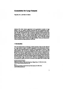
In Agronomy, it is usual to measure the soil penetration resistance in a region before sowing (Chan et al., 2006). Figure 1 shows 32 sampling locations in an experimental plot at the National University of Colombia, together with some penetration resistance profiles. For each sampling point, 334 observations of penetration resistance (MPa) were obtained on depths varying between 0 and 45 cm. The goal of analyzing this type of data is to predict penetration resistance on unsampled points based on the collected information, in order to carry out precision agriculture. If (classic) geostatistical methods are proposed to solve such prediction problem above mentioned, both multivariable kriging and space-time kriging techniques could be considered as alternative solutions to the functional approach. However, in the multivariable case, to estimate a coregionalization linear model (Wackernagel, 1995, 1998) with 334 variables is highly restrictive, and the space-time option is computationally very expensive to (finally) predict only one value of penetration resistance. A less flexi-
7
Geostatistics for functional data: An ordinary kriging approach
8
32 31
9800 17
30
9780
18
29
16
19
Latitude
9760
28
15
20
1
27
14
21
9740 2
26
13
22
3
9720
25
12
23
4 9700
11
24
5
10 6
9
9680
7 8
11100
11120
11140
11160
11180
11200
11220
11240
11260
11280
2.0
2.0
Longitude
1.5 1.0
Penetration resistance (MPa)
1.0
0.0
0.5
0.5
1.5
site 24 site 25
0.0
Penetration resistance (MPa)
site 1 site 16
0
10
20 Depth (cm)
30
40
0
10
20
30
40
Depth (cm)
Figure 1: Sampling points and some observed penetration resistance curves. Data are measured at the Marengo Experimental Station (National University of Colombia) during 2004. ble but easier alternative is to apply the prediction method proposed in this paper. To illustrate our approach, prediction on an unsampled location of the region is performed, together with a cross-validation analysis. The complete functional data set with 32 observed functions is shown in Figure 2. An outlier curve is clearly detected in this plot: that having values over 2.5 for depths in the range [30, 40] and corresponding to the sampling point with coordinates (11162, 9707) (point numbered as 4 in Figure 1). This outlying function was not considered in further analysis. The high variability observed in the empirical functions (Figure 2, left panel) suggested removing observational errors by using
Geostatistics for functional data: An ordinary kriging approach some smoothing technique. Consequently, smoothed curves of observed penetration resistance were obtained by using B-splines basis functions (see Figure 2, right panel). Spline functions are the most common choice for nonperiodic data (Ramsay and Silverman, 2005). Using the 31 remaining curves and the estimator in equation (6), the trace-semivariogram was calculated for several spatial lags. A spherical model was fitted to the estimated trace-semivariogram by using OLS technique (see Figure 3, left panel). The range of the fitted model was 110 meters, which can be interpreted, as in the classic geostatistical setting, that there is a strong spatial autocorrelation among the curves-note that the maximum distance between sampling points is 190 meters, and curves separated 110 meters are still correlated. Fitting a reasonable model to the trace-semivariogram is a critical step for subsequent interpolation of functional data by kriging. With the considered sampling scheme, it is not possible to have estimations of the trace-semivariance near to the origin, and thus it is possible that the nugget parameter was not well estimated. Consequently, it would be important to include more nearby sampling points in other essays in this experimental plot. As an example of the proposed methodology, kriging prediction on an unsampled location with coordinates 11179 (longitude) and 9750 (latitude) (see Figure 1) was performed. The kriging coefficients λ were obtained by solving the system in equation (4) with γ(h) estimated by the semivariance model given in Figure 3. The predicted curve (Figure 3, solid line in right panel) indicates that in this location there is a good soil compaction level, because the predicted penetration resistance is less than 2 MPa, which is considered the critical limit for root growth (Chan et al., 2006). We used cross-validation methods to compare observed and predicted curves. Crossvalidation was implemented by removing the curve χsi for each i, i = 1, · · · , 31, and further predicting χsi from the remaining data. A graphical comparison between observed and predicted curves (see Figure 4) shows that predicted curves are more smoothed than observed ones, as well as that the predicted data set has less vari-
9
2.0 1.5 0.5
1.0
Penetration resistance (MPa)
2.5 2.0 1.5 1.0 0.0
0.0
0.5
Penetration resistance (MPa)
10
2.5
Geostatistics for functional data: An ordinary kriging approach
0
10
20
30
0
40
10
20
30
40
Depth (cm)
Depth (m)
Figure 2: Set of 32 penetration resistance observed functions (left) and 31 smoothed functions (right). Smoothing on an outlier curve (see text) was not considered, and it is not showed in right panel. The dotted line in both panels indicates null penetration
0
2.0 1.5 0.0
0.5
1.0
4 2
Semivariance
6
Penetration resistance (Mpa)
8
2.5
resistance.
0
20
40
60
Distance (m)
80
100
0
10
20
30
40
Depth (cm)
Figure 3: Left panel: Spherical model fitted to the estimated trace-semivariogram: γˆ (h) = 8(1, 5h/110 − 0.5(h/110)3 ) for h ≤ 110 and γˆ (h) = 8 for h > 110. Right Panel: Measured curves of penetration resistance (dashed lines) and kriging prediction in an unsampled location (solid line). The dotted line in both panels indicates null penetration resistance. ance. This was not surprising since kriging is a smoothing method, and also because there is a significant high variability amongst penetration resistance values for some
1.5
Predictions (Mpa)
2.0
2.5
3.0
11
0.0
0.5
1.0
2.0 1.5 1.0 0.0
0.5
Penetration resistance (MPa)
2.5
3.0
Geostatistics for functional data: An ordinary kriging approach
0
10
20
30
40
0
10
20
Depth (cm)
30
40
Depth (cm)
Figure 4: Set of 31 penetration resistance (MPa) functions, obtained by B-spline smoothing (left), and predictions based on cross-validation (right). The dotted line in both panels
0.5 0.0 -0.5 -1.5
-1.0
Residuals (Mpa)
1.0
1.5
indicates null penetration resistance.
0
10
20
30
40
Depth (cm)
Figure 5: Cross-validation residuals (clear lines), residual mean (dark line) and residual standard deviation (dashed line). particular depth levels (see left panel of Figure 4). A detailed analysis of cross-validation residuals indicated that there was no evidence
Geostatistics for functional data: An ordinary kriging approach of biased predictions (see mean function in Figure 5). We also note that we had greater uncertainty on predictions both around 20 cm and greater than 40 cm of depth (see residual standard deviation in Figure 5).
5
Conclusions and further research
We have introduced an ordinary kriging predictor when data are curves. More complex procedures can be considered by replacing the scalar coefficients λi , i = 1, · · · , n in equation (1) by functional coefficients (λi (t), t ∈ T ), or even by double indexed functional coefficients (λi (s, t), s, t ∈ T ), and using integrals over T as a way to extend the definition of linear combinations. These extensions are parallel to regression models with functional responses (see, Chapters 14 and 16 in Ramsay and Silverman, 2005), and could be considered as extensions of the multivariable kriging predictor (Ver Hoef and Cressie, 1993) to the functional context. In this paper, and to analyze our data set, we have focused on B-splines, as a tentative smoothing technique, and on MoM and OLS techniques as classical estimation methods. However, further attention should be given to the use of: (a) other basis system to get functional data from discrete observations; (b) alternative methods of estimating the empirical trace-semivariogram, for instance, by using robust estimators (Cressie, 1993) or kernel estimation methods (Yu et al., 2007); (c) other parametric and nonparametric methods to fit the empirical trace-semivariogram; and (d) the automatic detection of outlier functions in the data set.
6
Appendix
The Appendix contains some detailed results mentioned in previous Section 2. A1. Solution of functional ordinary kriging based on trace-covariances.
12
Geostatistics for functional data: An ordinary kriging approach We need to minimize Z
13
n X ˆ s0 (t) − χs0 (t))dt + 2µ( V (χ λi − 1),
T
(7)
i=1
Pn
ˆ s0 (t) = i=1 λi χsi (t). The integral in equation (7) can be written as where χ Z 2 ˆ s0 (t) − χs0 (t))dt σs0 = V (χ ZT Z Z ˆ s0 (t))dt + ˆ s0 (t), χs0 (t))dt = V (χ V (χs0 (t))dt − 2 C(χ T
Z =
T
=
T
T
i=1
Z X n X n
−2
T i=1 n n XX
i=1
σ 2 (t)dt
λi λj C(χsi (t), χsj (t))dt +
T
λi C(χsi (t), χs0 (t))dt Z
λi λj
i=1 j=1
T
Z
T i=1 j=1 Z X n
=
T
Z Z n n X X 2 V( λi χsi (t))dt + σ (t)dt − 2 C( λi χsi (t), χs0 (t))dt
T
Z Cij (t)dt +
2
σ (t)dt − 2 T
n X
Z λi
i=1
T
Ci0 (t)dt.
(8)
Then, the objective function can be written as Z Z n n X n Z n X X X 2 λi λj Cij (t)dt + σ (t)dt − 2 Ci0 (t)dt + 2µ( λi − 1). (9) i=1 j=1
T
T
i=1
T
i=1
Minimizing (9) with respect to λ1 , · · · , λn and µ, we obtain the following set of (n + 1) equations n X j=1 n X
Z λj
T
Z C1j (t)dt + µ =
Z λj
T
j=1
T
C10 (t)dt
Z C2j (t)dt + µ =
T
C20 (t)dt
.. . n X j=1
Z λj
T
(10) Z
Cnj (t)dt + µ = n X j=1
λj = 1
T
Cn0 (t)dt
Geostatistics for functional data: An ordinary kriging approach
14
Now the result holds as equation (3) is a matrix notation of the system given in (10). A2. Solution based on the trace-semivariogram. We have, by using the notation given in Section 2, that γsi sj (t) = γ(χsi (t), χsj (t)) = V(χsi (t) − χsj (t)) 1 = E(χsi (t) − χsj (t))2 2 = σ 2 (t) − Cij (t). Then
Z T
Z Cij (t)dt =
Z 2
σ (t)dt − T
T
γsi sj (t)dt.
(11)
By replacing equation (11) in the system (10), we obtain the system given in equation (4). A3. The prediction trace-variance. From the first n equations in system (10), we have the relation n X n X
Z λi λj
i=1 i=1
T
Cij (t)dt =
n X
Z λi
T
i=1
Ci0 (t)dt −
n X
λi µ.
(12)
i=1
Replacing equation (12) into equation (8) we obtain Z 2
2
σ =
σ (t)dt − T
n X i=1
Z λi
T
Cio (t)dt − µ.
If, in addition, we consider the relation (11), we find the prediction tracevariance expression given in Section 2.
Acknowledgements Research partially supported by the Spanish Ministry of Education and Science and FEDER (MTM2004-06231 and MTM2006-09920) and by the EU PASCAL Network
Geostatistics for functional data: An ordinary kriging approach of Excellence (IST-2002-506778). We also would like to thank F. Leiva for providing his penetration resistance data set.
References [1] Cardot, H., Ferraty, F. and Sarda, P. (1999). Functional linear model. Statistics and Probability Letters, 45, 11–22. [2] Chan, K., Oates, A., Swan, A., Hayes, R., Dear, B. and Peoples, M. (2006). Agronomic consequences of tractor wheel compaction on a clay soil. Soil & Tillage Research, 89, 13–21. [3] Cressie, N.A.C. (1993). Statistics for Spatial Data. New York: John Wiley & Sons. [4] Deville, J. (1974). M´ethodes statistiques et numeriques de l´analyse harmonique. Ann. Insee, 15, 3–104. [5] Ferraty, F. and Vieu, P. (2003). Curves discrimination. A non parametric functional approaches. Computational Statistics & Data Analysis, 44, 161–173. [6] Ferraty, F. and Vieu, P. (2006). Non parametric functional data analysis. Theory and practice. New York: Springer. [7] Mancera, J. and Vidal, L. (1994). Florecimiento de microalgas relacionado con mortandad masiva de peces en el complejo lagunar Ci´enaga Grande de Santa Marta, Caribe colombiano. Anales del Instituto de Investigaciones Marinas, 23, 103–117. [8] Ramsay, J. and Silverman, B. (2005). Functional data analysis. Second edition. New York: Springer.
15
Geostatistics for functional data: An ordinary kriging approach [9] Silverman, B. (1995). Incorporating parametric effects into functional principal components. Journal Royal Statistical Society, Series B, 57, 673–689. [10] Tolosana-Delgado, R. (2005). Geostatistics for constrained variables. Positive data, compositions and probabilities. Applications to environmental hazard monitoring. Ph.D. Thesis, Universitat de Girona, Spain. [11] Ver Hoef, J. and Cressie, N.A.C (1993). Multivariable spatial prediction. Mathematical Geology, 25, 219–240. [12] Wackernagel, H. (1995). Multivariable geostatistics: An introduction with applications. Berlin: Springer-Verlag. [13] Wackernagel, H. (1998). Principal components analysis for autocorrelated data:
A geostatistical perspective. Technical Report 22/98/G, Centre de
Geostatistique-Ecole des Mines de Paris. [14] Wasserman, L. (2006). All of Nonparametric statistics. Berlin: Springer-Verlag. [15] Yu, K., Mateu, J. and Porcu, E. (2007). A kernel-based method for nonparametric estimations of variograms. Statistica Neerlandica, 61, 173–197.
16