Acoustics 08 Paris
Gesture synthesis: basic control of a flute physical model N. Montgermonta , B. Fabrea and P. De La Cuadrab a
Institut Jean Le Rond d’Alembert / LAM (UPMC / CNRS / Minist`ere Culture), 11, rue de Lourmel, 75015 Paris, France b Centro de Investigaci´on en Tecnologias de Audio (CITA), Universidad Cat´olica de Chile, Alameda 340, Oficina 13, Casilla 114-D Santiago, Chile
[email protected]
5697
Acoustics 08 Paris In the flute family, the oscillation is due to the instability of a jet at the output of a channel coupled with an acoustic resonator. Recent physical models allows to simulate the behavior of the complete instrument, but we still lack a convincing way to drive them. The simulation of the isolated instrument must be completed with a model of the control exerted by the flutist. Depending of the instrument of the flute family, the number and type of control parameters are different. For example, in a recorder the player blows inside a fixed channel built by the instrument maker and in the case of the transverse flute, the channel is shaped by the player’s lips during the playing. This paper presents a simple model of flute player, based on measurements carried on instrumentalists playing on a transverse flute. The model is generating the basic features of the instrument control in order to produce given pitches and dynamics. The coupling with a flute synthesis algorithm by physical modeling allows to study its validity.
1
Introduction
opening height hc . The distance between the lips opening and the edge of the labium is W and the transverse displacement of the is at a vertical distance ηW of the same point. The pipe is considered a one piece cylinder of constant radius a open on its extremity at a distance L of the labium.
Due to the complexity of the jet labium interaction, physical modeling of the flute instruments family is late compared to many instruments, piano and violin for example. Jet studies started with Rayleigh [9] in 1890. The first stationnary model of the jet drive coupled with a resonator was given by Cremer and Ising in 1968 [2] and an important improvement of the description of the recorder physics was done by Verge in 1995 [10]. Since these works, one direction is to extend the recorder model to the transverse Boehm flute as in De La Cuadra [3]. It leads to working synthesis algorithm that can be computed in real time on actual computers. The problem is the impressive amount of control parameters to drive the synthesis, even for such ”basic” task as playing one note: the complexity of the instrument is reflected in its digital representation. The aim of this paper is to introduce a model of the control exerted by the flutist at the entrance of existing synthesis by physical modeling algorithm. The solution presented here is based on measurements realized on real players in quasi normal playing conditions [8]. Section 2 describes the flute system and briefly explains the synthesis algorithm used for the instrument. Section 3 presents the model developed and Section 4 compared the data generated by a controlled flute model and measurements made on real players and discuss the pertinence of our work.
2
Figure 1: Side view of the flute model.
2.2
Lumped elements seems a good choice to simulate the behavior of the flute [4]. We use four elements calculated separately, the connections between them are presented at figure 2:
The flute system
The aim of this paper is not to discuss sound synthesis by physical modeling of a flute (see [3]). However, as explain before, the description of the instrument is necessary to understand the role of the instrumentalist. We recall here the more important points of actual algorithm and the choices we made.
2.1
Sound synthesis
Figure 2: Flute looped diagram.
The channel implements the conduct where the jet is formed. It computes the value uj of the jet center velocity regarding the pressure in the mouth of the instrumentalist pm using an incompressible fluid movement resulting in a Bernoulli equation [6]:
Model geometry
We choose to have a simple model that allows realtime computation but neglects some specific point of the transverse flute notably the angle of the jet towards the labium, the conicity of the first element of the resonator or the head joint. The transverse flute is modeled by extending the description developed by Verge [11] for the recorder. The lips of the players are seen as a conduct of length lc , with an opening surface towards the flute Sc and an
duj 1 + u2j (t) = pm (t) (1) dt 2 where ρ0 is the air density and the length lc is seen as a constant. ρ 0 lc
5698
Acoustics 08 Paris
2.4
The jet is the block computing the amplification and movement of the jet over the distance between the lips and the labium. It is the key part of the flute model and is the subject of many experiments. We choose here the empirical results of Cuadra et al. [3] that describes the jet using an exponential model. It is simplified to remove the frequency dependency of the jet response to the acoustic field. It allows us to compute the vertical position of the center of the jet ηW with ηW (t) = η0 (t − W/0.3uj )eαi W
In a recorder, the channel geometry is fixed by the instrument maker. The parameters Sc ,hc and W are thus constant and the control parameters are only the mouth pressure and the length of the pipe.
3 3.1
(2)
vW (t)hc (t) uj (t)
(3)
The sources are the aeroacoustic sources induced by the interaction between the jet and the labium. This element is modeled by a pressure dipole ∆p made by three different aeroacoustic sources. The main source is the acoustic field resulting of the jet oscillation interaction with the labium. It follows: ∆pj (t) = αW (t)
dqin dt
Flute player modeling Objectives
The aim of this work is to add a model of an instrumentalist in entrance of the instrument synthesis. We develop a model based on an analogy with simplified real flute performance. Reading a score, the musician, leaning on his technique, translate his musical intention into a set of parameters to play the instrument. We simplify the score by MIDI keyboard information: a pitch and a velocity. This will be the control of the instrumentalist we’ll had at the end . With these MIDI informations, the model must be able to compute a working set of control parameters to achieve a simple musical task: playing a note at a certain dynamic. As the musical tasks we want to command are very simples, we’ll refer to this part as “the playing technique”. As a first approach, the objective is only to control the static operation of the flute. No fine temporal control are used, and no model of attack or articulation between notes are developped here.
where αi is an empiric value and η0 is the perturbation at the origin given by: η0 (t) =
Recorder reduction
(4)
where αW is a value depending of the distance W and qin is the flow going inside the instrument, thus strongly depending of the jet position ηW . The two other sources are the turbulence induced by the interaction between the jet and the labium and the vortex shedding at the labium. See [10, 5, 3] for more details. The resonator block describes the acoustic field inside the resonator, specially the acoustic pressure pW and velocity vW at the entrance of the pipe. The models combines three different effects: • the propagation of plane waves along the pipe using the wave guide formalism • the visco-thermal losses caused by the inner walls of the pipe (see [7]).
Figure 3: Flutist modeling using two blocks.
• the radiation of a part of the wave at the extremity of the pipe.
2.3
3.2
Measurement regression
The model is divided in two parts as presented in Figure 3. The first part is based on measurements realized on flutists in real playing conditions. Control data as pm , W or Sc were collected with pressure sensors and a camera on 12 high level flutists. Amongst the set of data available, four parameters seemed to describe a complete state to achieve flute playing regarding the pitch and the dynamics [8]. These four relevant parameters has been chosen as a basis for the player model: L the pipe length, θ = uj /f W the dimensionless velocity, qj the jet flow at the lips opening and pm . A bi-dimensional regression is applied on the average measurements recorded on flutists playing scales at different dynamics. For each parameter γ we obtain a law of the form:
Input parameters
In order to drive the flute model, the following parameters must be given: • the pressure in the mouth of the instrumentalist pm • the mouth opening surface Sc • the mouth opening height hc • the distance between lips and labium W • the length of the pipe L
γ(f, d) = β0 + β1 f + β2 d + β3 f d
5699
(5)
Acoustics 08 Paris where γ is one of {θ, qj , pm }, f is the note to play (in Hz) and d the dynamic (in MIDI ranging from 0 to 127). The length of the pipe is determined by analogy with the real modern Boehm flute (see [1]). On the simplified instrument, the flutist plays the first mode of the resonator from C4 to C#5, then the second mode from D5 to C#6. For the highest octave the real fingerings make use of the third or fourth resonances in a complex way and no general rules can be written. We choose to extend the mechanism to the third octave, having the pipe played on its third resonance from D6 to C7. Finally, depending on the note to play: nc0 (6) L(f ) = 2f
The observations we made on the height of the channel shows that flutists maintain a quasi constant ratio between this value and Sc . hc is directly computed with p (10) hc = Sc /2 Finally, the pressure pm turns out to be to high to control our instrument model. A correction factor αmap has been empirically determined to correct the pressure pmap : pmap = αmap pm (11) with a value of αmap around 0.6.
3.4
where n ∈ {1, 2, 3}. This basic resonator will not be well tuned as to have the good pitch, you must include in your length the correction of the pipe extremity and tone holes, the visco thermal effects, and the covering of the embouchure by the instrumentalist. To play in tune is not important for the purpose of our synthesis. These results are presented for a part of the tessitura in Figure 4.
The modeling was implemented in the Pure Data software. This environment allows us to easily manage code, interface, audio device and MIDI control in real time. The flute model was developed in C as an external object and the player control was directly coded in the pd graphical language.
4
Mapping
The regression block manage the control of the length L of the resonator and pass a set of data to the mapping block to compute the others parameters. This block first calculate a desired jet velocity ujd r 2pm (7) ujd = ρ0
where Pxx (n) is the the Power Spectral Density at instant n and f0 is the frequency of the first note to play.
4.1
This value represents the stationnary velocity the flutist wants to obtain when he plays with the pressure pm . With this value we can compute the distance between the lips of the player and the labium: W = ujd /f θ
Playing of crescendo/diminuendo at a given pitch
The first task for comparison is a crescendo and diminuendo at a fixed pitch. The musician was asked to play the sequence on Figure 5 and the same task was commanded to the model by moving the velocity from 1 to 127 and back to 1 in 10 seconds with a given pitch. The descriptors are plotted on Figure 6.
(8)
and also the mouth opened surface. Sc = qj /ujd
Results and discussions
To discuss the interest of our model, we compare some real measurements to the coupling between the flute and the flutist models. A specific interest of the physical modeling is the great quality of the control one can apply to the instrument, therefore we choose to compare two tasks easily achieved with our model: a crescendo/diminuendo and an octave interval. The musician was asked to play the sequence and the pressure prad was recorded by a static microphone at a distance of approximately 1 m [?]. The same task was commanded to the model by controlling the pitch and the velocity. The value of the pressure at the entrance of the pipe pw was recorded during the operation. To simulate the radiation of the pipe from this pressure, we filtered the pression by a second order filter high pass filter cutting at 5kHz. The comparison is done on these two data by three perceptive representation of the signal. First, the amplitude of the signal is rapported to a sound pressure level decibel calculated on a 125ms window, then the spectrogram of the pressure is plotted and finally the evolution of the spectral centroid divided with the fundamental frequency is obtained with: P f (k)Pxx (k, n) (12) SCf0 (n) = k P f0 k Pxx (k, n)
Figure 4: Measured values (*) and regression (–) for L, θ, qj and pm for three dynamics(pp, mf, f f )
3.3
Implementation
(9)
5700
Acoustics 08 Paris quence a louder perceived sound.
4.2
Playing of octaves
Figure 5: crescendo/diminuendo at a slow tempo.
Figure 7: octave interval. The second task is the playing of octaves. The sequence played by the flutist is presented on the Figure 7 The model was ordered to play A4 with a velocity of 64 for 5 seconds and then to play A5 with the same velocity and for the same time. In order to play this interval, both the player and the model keeps the same resonator configuration and only play with the other parameters. The resulting data are shown on Figure 8.
Figure 6: Comparison between a crescendo/diminuendo realized by the synthesizer (up) and by a flutist (bottom). Are plotted the pressure amplitude in dBSP L , its spectrogram and its spectral centroid against the time. The first result is that the note is played by our synthesizer. The decibel scale shows that the pW pressure is louder than prad . Even if we know that the radiated pressure has a complexe pattern not implemented here, a difference of 20dB must indicate an overestimation of the sources. The amplitude of the synthesize signal is increasing by 7-8dB during the crescendo before to decrease to its initial value during the diminuendo. The two other parameters follows the evolution of the amplitude linearly and without fundamental change of the pressure shape. Analysis of the prad pressure shows two different strategies. First the evolution is nearly the same than the model, the amplitude evolves and the centroid slightly moves. But to achieve fortissimo playing, the flutist adopts a different way of increasing the loudness. The overall amplitude of the signal decreases a bit but the spectral centroid of the sound moves towards the higher frequencies increasing the second and third harmonics energy (≈ 1500 − 2300Hz). The human ear is much more sensitive to these frequencies having as a conse-
5701
Figure 8: Comparison between an octave interval realized by the synthesizer (up) and by a flutist (bottom). Are plotted the pressure amplitude in dBSP L , its spectrogram and its spectral centroid against the time. We recall that the spectral centroid is divided by the first frequency to play, A4 here. The model manage to play the interval as we can see with the pattern change on the spectrogram and with the centroid displacement. However, where the real player keeps a nearly constant amplitude, the model increase its pressure level of 15 dB when changing note. We can also see that the transition between the notes results in an impoverishment of the
Acoustics 08 Paris spectrum and a big variation of the centroid with the model where the player has a smooth evolution of both features.
[4] B. Fabre and A. Hirschberg. Physical modeling of flue instruments: a review of lumped models. Acustica united with Acta Acustica, 86:599–610, 2000.
[5] B. Fabre, A. Hirschberg, and A. Wijnands. Vortex shedding in steady oscillation of a flue organ pipe. Acustica united with Acta Acustica, 82:863– The player model we presented here manage to achieve 877, 1996. two simple musical tasks chosen to test it: a crescendo/diminuendo [6] N. Fletcher. Acoustical correlates of flute perforand an octave interval. It can control the production of mance technique. Journal of Acoustic Society of static notes with a quite good accuracy. However the America, 57:233–237, 1975. control it handles on the spectrum content of the sound is far from the quality of a human player. Where a [7] L. E. Kinsler. Fundamentals of Acoustics, third Ediplayer adapts and changes his strategies, the model is tion. 1982. only able to produce a set of data resulting of a mean of all the flutist recorded. [8] N. Montgermont, B. Fabre, and P. D. L. Cuadra. One direction to improve this work could be to anaFlute control parameters: fundamental techniques lyze the playing of one flutist and to identify the strateoverview. In International Symposium on Musical gies he employs when confronted to specific tasks. By Acoustics, 2007. this analysis, we could implement some fine temporal [9] J. Rayleigh. The Theory of Sound. Dover, 1896. control of the parameters, specially for the articulation between different notes. [10] M. P. Verge. Aeroacoustics of confined jets. PhD Adding a detection of the pitch and the loudness of thesis, TUE Eindhoven, 1995. the sound synthesized could be of great interest to feed this information back to the player model and to allow [11] M. P. Verge, B. Fabre, A. Hirschberg, and A. P. J. it to adjust the produced parameters. It will enhance Wijnands. Sound production in recorderlike instruthe homogeneity of the sound over all the tessitura of ments. i. dimensionless amplitude of the internal the instrument. Further developments also include a acoustic field. Journal of Acoustic Society of Amerfine modeling of the resonator to simulate the radiation ica, 101(5):2914–2924, Mai 1997. and to increase the quality of the synthesized spectrum. It will also enable a fine comparison between the two radiated pressure.
5
Conclusion
Acknowledgments The authors wants to thanks all the flutists that has been recorded, more specially : Robert Aitken, Michel Debost, Sophie Deshayes, Mark Fulep, Ricardo Ghiani, Shin-Ying Lin, Mikela Mann, Istvan Matuz and the students of the pedagogy course of the CNR of Versailles (C. Rayneau). They also thanks Claude Samuel and Diane de Rauquemaurel of the Rampal’s international concourse that has make the encounter with the participants and the jury possible. They also thanks the flute maker J.Y Roosen for the modifications he realized on the flute used for measurements. This work is partly supported by the ANR project Consonnes, directed by the LMA laboratory of Marseille.
References [1] T. Boehm. The Flute and Flute playing. Dover, 1964. [2] L. Cremer and H. Ising. Die selbsterregten schwingungen von orgelpfeifen. Acoustica, 19:143– 153, 1968. [3] P. de la Cuadra. The sound of oscillating air jets: physics, modeling and simulation in flute-like instruments. PhD thesis, Stanford, 2005.
5702