Getting Prime Cuts from Skylines over Partially Ordered Domains Wolf-Tilo Balke1, Ulrich Güntzer2, Wolf Siberski1 1
Forschungszentrum L3S Universität Hannover Appelstr. 4 30167 Hannover
[email protected] [email protected]
2
Institut für Informatik Universität Tübingen Sand 13 72076 Tübingen
[email protected]
Abstract: Skyline queries have recently received a lot of attention due to their intuitive query formulation: users can state preferences with respect to several attributes. Unlike numerical preferences, preferences over discrete value domains do not show an inherent total order, but have to rely on partial orders as stated by the user. In such orders typically many object values are incomparable, increasing the size of skyline sets significantly, and making their computation expensive. In this paper we explore how to enable interactive tasks like query refinement or relevance feedback by providing ‘prime cuts’. Prime cuts are interesting subsets of the full Pareto skyline, which give users a good overview over the skyline. They have to be small, efficient to compute, suitable for higher numbers of query predicates, and representative. The key to improved performance and reduced result set sizes is the relaxation of Pareto semantics to the concept of weak Pareto dominance. We argue that this relaxation yields intuitive results and show how it opens up the use of efficient and scalable query processing algorithms. Assessing the practical impact, our experiments show that our approach leads to lean result set sizes and outperforms Pareto skyline computations by up to two orders of magnitude.
1. Introduction Due to the ever growing volume of database content and the personalization needs in information searches, human preferences already play an essential part in today’s information systems. This is because mere SQLstyle queries only too often produce empty or too numerous results. First approaches at cooperative databases as those by [LL87, Mo88], handled user queries that retrieved empty results with respect to a database instance by automatic relaxation of query predicates. Using score values to express the utility of database objects with respect to a query, cooperative queries come in various flavors: • Top-k queries (see e.g. [GBK00, FLN01]) have shifted retrieval models from exact matching of attribute values to the notion of best matching database objects. Top-k models rely on basic scorings of objects for each query predicate and a utility function to aggregate the objects’ total scores.
•
•
Skyline queries extend this principle to cases where still score-based preferences exist for each query predicate, but no utility function is a-priori known to compromise between predicates (see e.g. [BKS01,TEO01,PTF03,BGZ04]). Skyline approaches adopt the principle of Pareto optimality, i.e. only those objects are returned, where no object exists in the database having better or equal predicate values. Multi-objective retrieval [BG04] finally allows for the interleaved evaluation of arbitrary compositions of skyline and top-k queries with proven instance-optimal complexity.
Especially the skyline paradigm has proven its usefulness in a variety of applications (e.g., digital item adaptation [KB06] or location-based services [HJ04]), since users generally cannot be expected to provide sensible weightings for a utility function. But while score-based approaches generally allow for efficient query evaluation, their expressiveness in terms of human user preferences remains rather limited, cf. [Fi99]. With the use of preferences modelled as strict partial orders with intuitive “I like A better than B” semantics ([Ch02, Ki02]), this lack of expressiveness was remedied at the price of more expensive query evaluation. A first evaluation algorithm of such partial order preference queries was given only recently by [CET05]. Also here the Pareto principle was used for evaluating queries involving several partial order preferences: • In [Ki02] and [CET05] a strong Pareto dominance principle called Pareto accumulation is used: an object has to be better or identical in all attribute values for the query predicates, and strictly better in at least one to dominate another object. • In contrast [Ch03] and [BG05] propose a weak Pareto dominance principle called Pareto composition, where an object’s attribute values has to be better, identical or incomparable in all predicates, and strictly better in at least one to dominate another object. The Pareto principle extends querying capabilities and the result set contains all possible best database objects with respect to arbitrary utility functions. On the other hand Pareto sets grow exponentially in size with increasing numbers of preferences [Be78]. Thus, typical tasks during the query process (like query refinement) rather need a good (and efficiently computed) overview over skylines. For instance, [KRR02] presents an online algorithm where users can influence the order in which skyline objects are produced. Eventually the entire skyline is calculated, but at every stage of the computation users can provide a direction where most relevant objects might be expected. The work in [BZG05] also relies on user interaction, by presenting the user with a representative sample of the expected skyline set, and then exploiting user feedback to elicit an appropriate utility function for the final result ranking. [KP05] proposes to cover the skyline set with ε-spheres where each center of a sphere is a representative for all skyline objects within a distance of at most ε. This set of representatives is subsequently returned to the user. However, the computation of an ε-sphere cover was shown to be NP-hard for more than 2 independent predicates. Moreover, the calculation of such approximations always needs expensive computations of the entire skyline. These approaches only focus on total-order preferences: all objects
can be compared in each predicate, which makes combinations of different predicates simple. Due to the indifference property in partial order preferences the Pareto combination leads to even bigger result sets: if an object is incomparable to other objects with respect to just a single preference, it still is Pareto-optimal and thus part of the skyline, even if it is the least preferred object with respect to all other preferences. In practical applications such incomparability often occurs: users can be indifferent between items and very rarely model preference relations between all possible attribute values for a query predicate anyway. Recent research in [Ki05] has started to combat such indifference in partial order preferences by means of ‘substitute values’. The substitute values (SV) semantics assigns equal usefulness to some incomparable values. Still, this semantics only remedies a small number of cases and is comparable in size and evaluation time to the complete skyline. Our goal is somewhat more ambitious. We want to efficiently provide ‘prime cuts’ of the skyline that can be used in an interactive query process. These prime cuts have to be both manageable in size and representative of the Pareto skyline. In this paper we present an innovative algorithm for the efficient computation of such prime cuts which relies on weak Pareto dominance, as defined in [BG05]. Weak Pareto dominance changes the preference semantics to an even higher degree than SV semantics. The resulting ‘restricted skyline’, i.e., all objects not weakly Pareto dominated, contains intuitively appealing objects, can be derived surprisingly efficient, and thus will deliver our prime cuts. The contribution of our approach is therefore twofold: • Restricted skylines derive manageable subsets of the partial order skylines (useful e.g. as a preview, or for query refinement) by taming the effects of incomparability. Our evaluation shows that sizes of restricted skylines are usually lean. • Our approach allows to efficiently approximate these restricted skylines without having to compute the entire Pareto set first. Query processing relies on progressive iteration of ranked result lists for each predicate and allows for pruning. In the following we will give a motivating scenario for partial order skylines and explain the semantics of the restricted skyline set. We will present the efficient evaluation algorithm for restricted skylines and perform extensive experiments to prove the practical applicability.
2. Weak Pareto Dominance and Restricted Skylines The following example will illustrate Pareto skylines and lead to the basic notion of weak Pareto dominance. Example 1: Given preferences P1 on car types and P2 on colors in Figure 1 and the following database instance: a green roadster, a black coupé, a blue SUV, a yellow truck and a pink limousine. None of them are dominated. The green roadster is maximal in P1. It does not dominate the black coupé, because black color is preferred over green. Furthermore, the user is indifferent between black and blue cars, thus the blue SUV is
red
roadster
black
coupé
blue grey
SUV truck
green
preference P1
preference P2
color
type
black
coupé
blue
SUV
green
roadster
pink
limousine
yellow truck database instance
Figure 1. Partial order preference example
not dominated by the black coupe, nor dominated by the green roadster because of P2. Though the yellow truck has the worst car type, the user has not given any judgment on its color, thus making it incomparable. Finally, the pink limousine is completely incomparable to all other objects. Thus, the Pareto skyline contains all five elements. Using the normal definition of Pareto sets, in Example 1 the entire database would have to be retrieved and returned to the user. Since a user usually is interested in refining queries according to the most promising result objects, retrieving a sophisticated selection from the skyline is a far more cooperative behavior. Our restricted skyline is such a selection. But on what grounds can we select ‘better’ objects from the full Pareto skyline? Generally speaking, skyline queries are only sensible if no ordering or weightings between individual predicates are provided. Otherwise utility-based ranking schemes such as top-k queries would be far more efficient to use. Pareto sets are designed to consist of all optimal objects with respect to all possible utility functions. Therefore, selecting a subset of the skyline will always ignore objects that are nevertheless optimal for some utility function. In other words, any selection will consider some utility functions as being more probable than others. Such an assessment has to be based on heuristics. We rely on the heuristic that all user preferences should be relaxed evenly and as little as possible, i.e. the relaxation scheme should be fair. In any case, a selection doesn’t have to be the final result set. If it can be computed reasonably fast and yields manageable result sets, it can also be used as a good starting point for focused searches such as the online algorithm in [KRR02] or the feedback algorithm in [BZG05]. Since our selection relies on weak Pareto dominance, we will formalize its semantics in the following definition (cf. Pareto composition in [Ch03]): Definition 1: (weak Pareto dominance) Let O be a set of database objects and x, y ∈ O. An object x is said to weakly dominate object y with respect to partial order preferences P1, …, Pn, if and only if there is an index i (1 ≤ i ≤ n) such that x dominates y with respect to Pi and there is no index j (1 ≤ j ≤ n) such that y dominates x with respect to Pj. That means, with >P denoting the domination with respect to partial order P: x weakly dominates y ∃ i (1 ≤ i ≤ n): x >Pi y ∧ ¬∃ j (1 ≤ j ≤ n): y >Pj x We call the set of all non-weakly-dominated objects the ‘restricted’ skyline. Please note that for total order preferences, weak and strong Pareto dominance coincide, because
green roadster
pink limousine
black coupé
blue SUV
yellow truck
Figure 2. Sample weak dominance graph
there are no incomparable objects. Let us reconsider our example and see what changes, if we restrict the skyline set using weak Pareto dominance. Example 1 (cont.): Consider the objects from above under the notion of weak Pareto dominance (Figure 2). There is still no weak dominance relation between the green roadster, and the black coupé, because black color is preferred to green, but a roadster is deemed better than a coupé. However, both of them now weakly dominate the yellow truck and it can be removed in the restricted skyline. Removing the yellow truck seems indeed a very intuitive thing to do, because P1 tells us that everything is better than a truck and the user, although voicing explicit color preferences, did not express his/her opinions on yellow cars. Moreover, we have to take a closer look at the relation between the black coupé and the blue SUV. The user is indifferent between both colors. But the black coupé fits his/her car type wishes to a higher degree, hence is probably more desirable. The weak dominance relation reflects this semantics: the blue SUV is weakly dominated by the black coupé and can be removed. Please note that the pink limousine with incomparable predicate values only is still not dominated by anything and will thus also be part of the restricted skyline. This reflects the notion that an item may be desirable, even if a user was not aware of it when formulating the query. In the end, the result size in our small example is almost halved and only less intuitive candidates have been pruned. Our work in [BG05] shows that restricted skylines are a proper subset of the normal skyline, i.e. the strong Pareto set. The same applies to the substitute values skyline, as shown in [Ki05]. Finally, it can be shown that the restricted skyline is always a subset of the SV-skyline.
3. Efficiently Computing Restricted Skylines Unlike numerical skylines, any partial order algorithm needs to handle object incomparability. This makes algorithms on total orders (such as NN [KRR02] and BBS [PTF03]) unsuitable. In contrast we rely on a scheme using topologically ordered lists: for each query predicate a list of all database objects sorted according to the respective user preference is created. Incomparability can be resolved by exploiting the level order of the preference. The algorithm’s main challenge is to determine, if all relevant objects have already been seen. In each query evaluation our algorithm therefore first computes possible value combinations (so-called l-cuts), which guarantee safe pruning: if a set of
red
Level 1 Level 2
black blue grey
Level 3 green
Level 4
preference P2
Figure 3. Level order example
objects instantiate any l-cut no relevant object can exist in the tails (higher than level l) of the sorted lists. The creation of the sorted lists and the calculation of the pruning thresholds are only dependent on preference size, not on database size, and therefore fast to compute. 3.1 Level Order for Partial Order Preferences For pruning, we have to arrange for sorted access to objects for each query predicate: possibly relevant objects should be returned earlier than rather irrelevant objects. To create a proper sorting from the given partial preference orders, we use a simple breadth first topological ordering defining ‘levels’: Definition 2: (level order) Let P be a partial order preference. A value v is said to belong to level l or level(v) = l with respect to P, if and only if the longest path from any maximum attribute value in P to v consists of (l - 1) edges. Values not explicitly expressed in P belong to level 1. We denote the set of all values in level l as levell := {v | level(v) = l}. Analogously, a database object x is said to be in level l with respect to P, iff its attribute value is in level l. This notion of levels imposes an intuitive sorting: all maximum (i.e. non-dominated) objects of P are on level 1, all objects that are only dominated in P by maximum objects are on level 2, and so on. We call this order level order. In the special case of numerical or total order preferences the level corresponds to each object’s rank, if objects with identical scores/attribute values are considered to have equal rank. But for partial orders this level order has another nice property: Lemma 1: (level order domination) Let O be a set of database objects and x, y ∈ O. Then object x can only dominate object y with respect to a partial order preference P, if level(x) < level(y) with respect to P. Proof: If x dominates y there is a path of length q > 0 from x to y in P. Thus it directly follows from the definition of levels by longest paths in Definition 2, that: level(x) < level(x) + q ≤ level(y). ■
Though objects can only be dominated by objects in smaller levels, due to the partial order semantics they do not have to be dominated by all objects in these levels, but can also be incomparable. For example, blue cars are in a smaller level than grey cars for our preference P2, although both are incomparable (see Figure 3). In the following we will assume all database objects to be accessed in level order for each preference. Note that it is not necessary to compute a complete object index based on the level order for each incoming query. Instead, the database maintains object sets clustered by value, i.e., the sets of objects sharing the same value for a predicate. Then, creating a list in level order just means to sort references to these sets, not to sort all database objects. Since user preferences are typically rather small, producing level orders is fast even for large databases. 3.2 Identifying the Pruning Thresholds In the last section we have defined a sorted list of objects for each predicate. For pruning we introduce the concept of l-cuts. While iterating over the lists, we have to check whether all relevant (i.e. not weakly dominated) objects have been accessed already. Definition 3: (l-cut of preference orders) For a partial order preference P and natural number l, a subset of values C ⊆ P is called l-cut, if (a) ∀ v ∈ C : level(v) ≤ l (b) ∀ (w ∈ P\C) ∃ v ∈ C : v >P w A set of database objects D forms an instance of an l-cut C if for each v ∈ C ∃ o ∈ D: o has attribute value v. An l-cut C is minimal, if no subset C’ ⊂ C is an l-cut. The intuitive meaning of l-cuts is to form sets of attribute values that if instantiated by database objects, dominate all object values beyond the l-th level. Every completely instantiated level of values forms a trivial l-cut. But generally l-cuts will be much smaller, and in the following we only need to consider minimum l-cuts. Example 1 (cont.): Every single red car is instance of a 1-cut with respect to P2. A 2-cut is instantiated by any pair of a blue and a black car. Regarding preference P1, every roadster is instance of the 1-cut, every coupé instantiates a 2-cut, and so on. For efficient pruning in our skyline evaluation we have to allow for quick tests whether a set of objects instantiating an l-cut has already been accessed. Hence, our first step in query evaluation is to compute all minimal l-cuts for each preference dimension. If we later find some object set instantiating any such cut we have found a pruning threshold. We now present a simple way to calculate minimal l-cuts. We first split the preference graph into levels, according to Definition 2:
Algorithm 1 (calculating attribute value levels) 0. Select level1 as the set of all maximum attribute values in a preference graph P, i.e. all attribute values that are not dominated by any other attribute value. l := 1 1. levell+1 := ∅ 2. While there are attribute values in levell do 2.1. Consider the next attribute value x in levell 2.2. For each attribute value y directly dominated by attribute value x with respect to P do 2.2.1. If y ∉ level0 ∪…∪ levell +1, then levell +1 := levell +1 ∪ {y} 2.2.2. If y ∈ levelj for some j ≤ l, then remove y from levelj and set levell+1 := levell+1 ∪ {y} 3. If levell+1 is not empty, set l := l+1 and proceed with step 1. From these level sets, we can now determine minimal l-cuts. Obviously, each complete set levell is a cut candidate, because all objects having attribute values in levelj with l < j are dominated by some object having an attribute value from set levell. Moreover, if we replace some cut element by any object dominating that cut element, the resulting set still forms a cut. Thus, to find all possible cut candidate value sets, we have to systematically enumerate all possible replacements. For this purpose, we first build a cut candidate value set from each complete levell and then exhaustively replace attribute values by dominating values. Finally we remove redundant values to identify minimal cuts. Algorithm 2 (calculating minimal cut value sets) 0. Given n sets of attribute values level1 ,…, leveln as output by algorithm 1 and initialize candidates1,…, candidatesn := ∅, replace1,…, replacen := ∅ and minimalcuts1,…, minimalcutsn := ∅. 1. For l := 1 to n do 1.1. If levell ∉ candidatesl then candidatesl := candidatesl ∪ {levell} 1.2. For j := 1 to |levell| do 1.2.1. Consider the j-th attribute value aj in an enumeration of levell and initialize replacej := ai 1.2.2. For each y with aj