ing other Bayesian advantages (mitigation of data sparseness prob- lems and ..... speaker clustering experiments by using the TIMIT development and core sets ...
GIBBS SAMPLING BASED MULTI-SCALE MIXTURE MODEL FOR SPEAKER CLUSTERING Shinji Watanabe, Daichi Mochihashi, Takaaki Hori, and Atsushi Nakamura NTT Communication Science Laboratories, NTT Corporation 2-4, Hikaridai, Seika-cho, Soraku-gun, Kyoto, 619-0237, Japan ABSTRACT The aim of this work is to apply a sampling approach to speech modeling, and propose a Gibbs sampling based Multi-scale Mixture Model (M3 ). The proposed approach focuses on the multi-scale property of speech dynamics, i.e., dynamics in speech can be observed on, for instance, short-time acoustical, linguistic-segmental, and utterance-wise temporal scales. M3 is an extension of the Gaussian mixture model and is considered a hierarchical mixture model, where mixture components in each time scale will change at intervals of the corresponding time unit. We derive a fully Bayesian treatment of the multi-scale mixture model based on Gibbs sampling. The advantage of the proposed model is that each speaker cluster can be precisely modeled based on the Gaussian mixture model unlike conventional single-Gaussian based speaker clustering (e.g., using the Bayesian Information Criterion (BIC)). In addition, Gibbs sampling offers the potential to avoid a serious local optimum problem. Speaker clustering experiments confirmed these advantages and obtained a significant improvement over the conventional BIC based approaches. Index Terms— Fully Bayesian approach, Gibbs sampling, multi-scale mixture model, Gaussian mixture, speaker clustering 1. INTRODUCTION Statistical modeling plays an essential role in the processing of realworld data such as text, speech and images. An important aspect of this modeling technique is the consideration of the multi-scale property in dynamics within a probabilistic framework. For example, Probabilistic Latent Semantic Analysis (PLSA) is a successful approach in terms of the multi-scale property, which accurately deals with two types of scales, namely, word-level and document-level scales, based on a latent topic model [1]. In addition, Latent Dirichlet Allocation (LDA) [2] realizes the fully Bayesian treatment of the latent topic model. Consequently, the latent topic model is connected to Bayesian statistics and machine learning fields, and is further extended by using various techniques developed in these fields (e.g. hierarchical Dirichlet processes [3]). This paper is inspired by these successful approaches, and aims to apply a fully Bayesian treatment to the multi-scale properties of speech dynamics. There have been certain studies on Bayesian speech modeling, e.g., by using Maximum A Posteriori (MAP) or Variational Bayesian (VB) approaches for speech recognition [4, 5], speaker recognition [6], and speaker clustering [7]. While all of these approaches are based on the EM-type deterministic algorithm, this paper focuses on another method of realizing fully Bayesian treatment, namely sampling approaches. The main advantage of the sampling approaches is that they can avoid local optimum problems in addition to providing other Bayesian advantages (mitigation of data sparseness problems and capability of model structure optimization). While their heavy computational cost could be a problem in realization, recent improvements in computational power and the development of theoretical and practical aspects related to the sampling approaches allow
978-1-4577-0539-7/11/$26.00 ©2011 IEEE
4524
us to apply them to practical problems (e.g., [8,9] in natural language processing). Therefore, the aim of this work is to apply a sampling approach to speech modeling considering the multi-scale properties of speech dynamics. In this paper, as an analogy with the document and word units in LDA, we focus on two kinds of temporal scales corresponding to two kinds of speech dynamics, which might be observed by shorttime or “frame”-based analysis with a period of a few dozen milliseconds, and which might occur with utterance-wise periods, respectively. The former (frame-level dynamics, hereafter) is mainly due to phonological succession in speech content, the existence of non-stationary noise, etc., while the latter (utterance-level dynamics, hereafter) is mainly driven by changes of speakers, emotional states, topics, etc., over time. We use conventional Gaussian Mixture Models (GMMs) for the frame-level speech dynamics as continuous density models, and a mixture of these GMMs for the utterancelevel speech dynamics. Thus, the model can appropriately cluster the frame-level and utterance level speech variations simultaneously, unlike the BIC based single Gaussian model [10], which can only model the utterance level dynamics. We call this the Multi-scale Mixture Model (M3 ). M3 is a simple and effective model representation for use in GMM-based speaker recognition and clustering [6, 7, 11], and it can be extended to a hidden Markov model in speech recognition by considering piecewise stationary dynamics on a segment-level time scale rather than an utterance-level time scale. One of the difficulties for M3 is that it is not easy to obtain the utterance clustering criterion (measure) due to the complicated representation of an utterance. For example, the Kullback-Leibler divergence between GMMs cannot be computed analytically, and some approximation is required [11]. Another difficulty is that such kinds of hierarchical mixture models are severely affected by a local optimum problem. To overcome these difficulties, we propose a sampling-based fully Bayesian realization of M3 , and cluster the frame-level and utterance-level speech variations by consistently using the Bayesian criterion. This paper provides an analytical solution based on Gibbs sampling, which jointly infers the mixture variables by interleaving frame-level and utterance-level samples. This can be applied to various unsupervised clustering tasks in speech processing, e.g., phonetic decision tree clustering for context-dependent hidden Markov model and speaker clustering. We describe speaker clustering experiments that proved to yield a significant improvement compared with the conventional BIC based approaches thanks to these advantages.
2. FORMULATION This section formulates the multi-scale mixture model (M3 ) by utilizing a Gibbs sampling. Section 2.1 introduces M3 , and Section 2.2 provides its generative process and the graphical model. Section 2.3 derives the marginalized likelihood of M3 , which is used for deriving Gibbs samplers in Section 2.4.
ICASSP 2011
2.1. Multi-scale mixture model M3 considers the two types of observation vector sequences. One is an utterance- (or segment) level sequence and the other is a framelevel sequence. Then, a D dimensional observation vector (e.g. MFCC) at frame t in utterance u is represented as ou,t (∈ RD ). A set of observation vectors in utterance u is represented as ou , u {ou,t }Tt=1 . Then, we assume that the frame-level sequence is modeled by a Gaussian Mixture Model (GMM) as usual, and the utterance-level sequence is modeled by a mixture of these GMMs. Two kinds of latent variables are involved in M3 for each sequence: utterance-level latent variable zu and frame-level latent variable vu,t . Utterancelevel latent variables may represent emotion, topic, and speaking style as well as speakers, depending on the speech variation. The likelihood function of U observation vectors (O , {ou }U u=1 ) given the latent variable sequences (Z , {zu }u and V , {vu,t }u,t ) can be expressed as follows: p(O|Z, V, Θ) =
U Y u=1
hz u
Tu Y
Utterance level weight Frame level weight
(1) where {hs }s , {ws,k }s,k , {—s,k }s,k , {Σs,k }s,k (, Θ) are the utterancelevel mixture weight, frame-level mixture weight, mean vector, and covariance matrix parameters, respectively. s and k denote utterance and frame level mixture indexes, respectively. N denotes a Normal distribution.
Frame-level latent variable Feature vector
Mean Covariance
Frame index Utterance index Frame-level mixture index
Fig. 1. model.
Utterance-level mixture index
Graphical model representation of multi-scale mixture (b) For each frame t = 1, · · · , Tu i. Draw vu,t from Multinomial (wzu ) ii. Draw ou,t from Normal (—zu ,vu,t , Σzu ,vu,t )
wzu ,vu,t N (ou,t |—zu ,vu,t , Σzu ,vu,t ),
t=1
Utterance-level latent variable
The corresponding graphical model is shown in Figure 1. Now we have introduced M3 , the following sections derive a solution for M3 based on Gibbs sampling.
2.3. Marginalized likelihood for the complete data In a Bayesian inference framework, we focus on the marginalized likelihood for the complete data. In the complete data case, all of 2.2. Generative process and graphical model the latent variables are treated as observations, i.e., the assignments We consider the Bayesian treatment of this multi-scale mixture of the all latent variables are hypothesized to be given in advance. model. We assume a diagonal covariance matrix for the Gaussian Then, p(zu = s|·) , δ(u, s) and p(vu,t = k|·) , δ(u, t, k) return 0 distributions as usual1 where the d-d diagonal element of the covarior 1 based on the assignment information, and the sufficient statistics ance matrix is expressed as σdd . We also assume that the prior hyperof M3 can be represented as follows: parameters of the GMM parameters ({ws,k }s,k , {—s,k }s,k , {Σs,k }s,k ) P 8 cs = u δ(u, s), for each s are shared with the parameters of one GMM (universal > P > > P : jugate distributions are used as the prior distributions of the model rs,k,dd = u,t δ(u, s)δ(u, t, k)(ou,t,d )2 . parameters: 9 8 cs is a count of utterances assigned to s and ns,k is a count of frames h ∼ D(h0 ) > > assigned to k in s. ms,k and rs,k,dd are 1st order and 2nd order > > = < 0 ∼ D(w ) ws sufficient statistics, respectively. , (2) p(Θ|Ψ0 ) = 0 0 −1 ∼ N (— , (ξ ) Σ ) — Based on the sufficient statistics, the likelihood for the complete > > s,k k s,k > > ; : 0 data can be expressed as follows: (σs,k,dd )−1 ∼ G(η 0 , σk,dd ) 0 where h0 , w0 , —0k , ξ 0 , σk,dd , η 0 (, Ψ0 ) are the hyper-parameters. D and G denote Dirichlet and Gamma distributions, respectively. Based on the likelihood function and prior distributions, the generative process of M3 can be expressed as follows: 1. Initialize Ψ0 2. Draw h from Dirichlet (h0 ) 3. For each utterance-level mixture component s = 1, · · · , S
p(O, Z, V|Θ) Y Y Y (hs )cs (ws,k )ns,k δ(u, s)δ(u, t, k)N (ou,t |—s,k , Σs,k ). = s
k
u,t
(4)
The marginalized likelihood for the complete data, p(O, Z, V|Ψ0 ), can be obtained analytically as shown below by substituting Eqs. (2) and (4) into the following integration.
(a) Draw ws from Dirichlet (w0 ) (b) For each frame-level mixture component k = 1, · · · , K i. For each dimension d = 1, · · · , D 0 A. Draw (σs,k,dd )−1 from Gamma (η 0 , σk,dd ) ii. Draw —s,k from Normal (—0k , (ξ)−1 Σs,k ) 4. For each utterance u = 1, · · · , U (a) Draw zu from Multinomial (h) 1 If
we consider the full-covariance matrix, its conjugate distribution becomes a Wishart distribution.
4525
p(O, Z, V|Ψ0 ) Z = p(O, Z, V|Θ)p(Θ|Ψ0 )dΘ P 0 Q ˜ s ) Y Γ(P wk0 ) Q Γ(w Γ( hs ) s Γ(h ˜s,k ) k Q k 0 P = Q s 0 P ˜ Γ(h ) Γ(w ) Γ( w s Γ( k s k k ˜s,k ) s hs ) s “ “ ”” −D`Q ´ η0 0 D 0 2 (ξ 0 ) 2 Γ η2 σ Y − ns,k D k,dd d 2 (π) , · “ “ ””−D`Q ´ η˜s,k D η ˜ 2 s,k (ξ˜s,k ) 2 Γ s,k σ ˜ s,k,dd d 2 (5)
˜s, w ˜ are the hyper˜ s, — ˜ s,k , ξ˜s,k , σ where h ˜s,k,dd , and η˜s,k (, Ψ) parameters of the posterior distributions for Θ, which are obtained from the hyper-parameters of the prior distributions (Ψ0 ) and sufficient statistics (Eq. (3)) as follows: 8 ˜s > h = h0s + cs , > > > > ˜s,k = wk0 + ns,k , >w > > ˜ < ξs,k = ξ 0 + ns,k , (6) ξ 0 —0 k +ms,k > μ ˜ = , > ξ˜s,k > s,k > > > = η 0 + ns,k , η˜s,k > > : 0 σ ˜s,k,dd = σk,dd + rs,k,dd + ξ 0 (μ0k,d )2 − ξ˜s,k (˜ μs,k,d )2 . Based on the marginalized likelihood for these complete data, we calculate the conditional distribution of vu,t and zu , as shown below. 2.4. Gibbs sampler [Frame-level mixture component] The Gibbs sampler assigns frame-level mixture component k at frame t by using the following equation: log p(vu,t = k|O, V\t , Z\u , zu = s) « „ p(O, V\t , vu,t = k, Z\u , zu = s) , ∝ log p(O\t , V\t , Z\u , zu = s) ˜ s,k ) − gs,k (Ψ ˜ s,k\t ). ∝ gs,k (Ψ
1: Initialize Φ0 2: repeat 3: for u = shuffle (1 · · · U ) do 4: for t = shuffle (1 · · · Tu ) do 5: Sample vu,t by using Eq. (7) 6: end for 7: end for 8: for u = shuffle (1 · · · U ) do 9: Sample zu by using Eq. (8) 10: end for 11: until some condition is met
O\u and V\u . Therefore, the posterior probability can be obtained as follows: p(zu = s� |O, V, Z\u ) P ” “ P Γ( w ˜ � ) ˜ s� ,k ) − gs� ,k (Ψ ˜ s� \u,k ) � ,k (Ψ + g exp log Γ(Pk ws˜ \u,k s k � ,k ) “ k Γ(sP ” . = P ˜s\u,k ) kw ˜ s,k ) − gs,k (Ψ ˜ s\u,k ) P exp log + gs,k (Ψ s,k Γ( w ˜s,k ) k
(8)
Thus, we can derive a solution for the multi-scale mixture model based on Gibbs sampling, which jointly infers the latent variables by interleaving frame-level and utterance-level samples. Algorithm 1 provides a sample code of the proposed approach.
Here, O\t and V\t indicate sets that do not include the tth frame elements. Z\u indicates a set that does not include the uth utterance ˜ s,k\t is computed by the sufficient statistics using O\t element. Ψ and V\t . gs,k (·) is defined as follows: D ˜ s,k ) , log Γ(w gs,k (Ψ ˜s,k ) − log ξ˜s,k „ 2« η˜s,k X η˜s,k − + D log Γ log σ ˜s,k,dd . 2 2 d
Therefore, by considering the normalization constant, the posterior probability can be obtained as follows: p(vu,t = k� |O, V\t , Z\u , zu = s) ” “ ˜ s,k� ) − gs,k� (Ψ ˜ s,k� \t ) exp gs,k� (Ψ “ ”. = P ˜ ˜ k exp gs,k (Ψs,k ) − gs,k (Ψs,k\t )
Algorithm 1 Gibbs sampling based multi-scale mixture model.
(7)
This equation is analytically derived by using the marginalized likelihood for complete data (Eq. (5)). [Utterance-level mixture component] As with the frame-level mixture component case, the Gibbs sampler assigns utterance-level mixture s at utterance u by using the following equation: log p(zu = s|O, V, Z\u ) « „ p(O, V, Z\u , zu = s) ∝ log p(O\u , V\u , Z\u ) P Γ( k w ˜ ) X ˜ s,k ) − gs,k (Ψ ˜ s\u,k ). P s\u,k + ∝ log gs,k (Ψ Γ( k w ˜s,k ) k
O\u and V\u indicate sets that do not include subsets of the frame ˜ s\u,k is computed by the sufficient statistics using elements in u. Ψ
3. EXPERIMENTS FOR SPEAKER CLUSTERING We applied the proposed approach to speaker clustering tasks to demonstrate its effectiveness. We used the TIMIT database, and also more realistic speech data, namely meeting conversations. 3.1. Experimental results for TIMIT As an observation vector, we used MFCC features with log energy, Δ, and ΔΔ components. First, a prior GMM (i.e., universal background model) was estimated by using a TIMIT training set consisting of 3,696 utterances based on the conventional ML-EM algorithm, and the values of the GMM parameters were set as those of the hyper-parameters in M3 (w0 , —0k , Σ0k ). We prepared two sets of speaker clustering experiments by using the TIMIT development and core sets, respectively. The development set consisted of 144 speakers × 8 utterances, and the core set consisted of 24 speakers × 8 utterances. As a preliminary experiment, the numbers of clusters were set at the correct answer. The number of Gaussian mixture components and the values of the other hyper-parameters (h0 , ξ 0 , η 0 ) were determined by using the speaker clustering performance of the development set. The speaker clustering performance was measured in terms of the geometric mean of the cluster and speaker purities introduced in [7, 13], where the speaker label for each utterance and the utterance interval were manually annotated in the all experiments. The number of iteration counts was set at 50, and the initial values of the frame-level and utterance-level latent variables were randomly assigned. Table 1 shows the speaker clustering performance of the proposed approach (M3 Gibbs), the MAP based approach (M3 MAPEM), and the conventional BIC based approach [10]. Speaker clustering experiments showed that M3 Gibbs provided a significant improvement over the conventional BIC and M3 MAP-EM based approaches. The main advantage of M3 Gibbs and M3 MAP-EM over BIC is that these can precisely model speaker clusters based on the Gaussian mixture model unlike the single Gaussian model used in BIC. In addition, M3 Gibbs further improved on the speaker clustering performance of M3 MAP-EM since the Gibbs sampling algorithm in the proposed approach can avoid local optimum solutions
4526
unlike the MAP-EM algorithm. These superiorities are derived from the Gibbs based Bayesian properties of the proposed approach. 3.2. Experimental results for meeting data We also applied the proposed approach to meeting data, which was recorded by NTT Communication Science Laboratories to analyze and recognize meetings [14]. We used 6 meeting sessions. We used 4 of the sessions (3,402 utterances) for constructing a prior GMM in advance, and the other 2 sessions as development (495 utterances spoken by 4 speakers) and evaluation sets (560 utterances spoken by 4 speakers), respectively. The experimental setup was same as that used for the TIMIT experiments. Table 2 shows the speaker clustering performance of the proposed approach (M3 Gibbs), the MAP based approach (M3 MAPEM) and the conventional BIC based approach. In addition, Table 2 also provides the frame-level error rate of each method based on the diarization error rate defined by NIST [15] as another performance measure of speaker clustering. The proposed approach also provided significant improvements over the conventional approaches for both performance measures. Thus, these two experimental tasks show the effectiveness of the proposed approach. 3.3. Computational cost We finally discuss computational cost. One of the most serious problems that has prevented sampling based approaches from being widely used for speech modeling is computational cost. P For example, compared with the quadratic form ( d (ot,d − μs,k,d )2 (σs,k,dd )−1 ) of frame-wise likelihood computation required for the maximum likelihood, MAP and VB approaches2 , the proposed approach uses Eq. (7) and requires heavy computation due to logarithmic (log) and gamma (Γ) functions. Because the proposed approach was straightforwardly implemented without considering fast computation techniques, it was several times slower than the EM-based approaches when using our computers (Intel Xeon X5570 2.93 GHz). However, in the TIMIT development set experiments (1,152 utterances, 3,530 seconds), the proposed approach took an average of only about 23 seconds for one epoch of iterative calculation. Therefore, it is practical for use in speaker clustering tasks. If we increase the model size e.g., by applying it to acoustic models in speech recognition, the computational cost will increase greatly. However, many techniques have recently been developed for efficient computation with sampling approaches (e.g., blocked Gibbs, beam sampling, GPU computation, independence assumption and parallelization), which enable us to realize large-scale speech modeling based on sampling techniques. 4. SUMMARY This paper proposed a Gibbs sampling based Multi-scale Mixture Model (M3 ) and applied it to a speaker clustering task. Preliminary experiments confirmed the effectiveness of the proposed approach by comparison with the conventional BIC based approaches. One of the characteristics of the proposed approach is that we can derive a fully Bayesian treatment of multi-scale speech dynamics. Therefore, Table 1. Experimental results for TIMIT Method BIC M3 MAP-EM M3 Gibbs BIC M3 MAP-EM M3 Gibbs
(Dev.) (Dev.) (Dev.) (Eval.) (Eval.) (Eval.)
cluster purity 0.466 0.524 0.725 0.715 0.791 0.895
speaker purity 0.460 0.389 0.601 0.655 0.624 0.797
we will apply some recently developed Bayesian approaches to the proposed approach (e.g., Dirichlet process mixtures [3] for model structure (frame and utterance level mixture sizes) optimization). In addition, one of our goals is to model whole spoken language processing (e.g., speech recognition and understanding) by using sampling approaches. Therefore, we will extend our approach to a continuous density hidden Markov model for speech recognition, similarly to MAP and VB approaches [4, 5]. We also envision combining our approach and Bayesian language modeling (e.g., [9]) to realize a fully Bayesian treatment of acoustic and language modeling in spoken language processing. 5. REFERENCES [1] T. Hofmann, “Probabilistic latent semantic analysis,” in Proc. UAI’99, 1999, pp. 289–296. [2] D. M. Blei, A. Y. Ng, and M. I. Jordan, “Latent Dirichlet allocation.,” Journal of Machine Learning Research, vol. 3, pp. 993–1022, 2003. [3] Y.W. Teh, M.I. Jordan, M.J. Beal, and D.M. Blei, “Hierarchical Dirichlet processes,” Journal of the American Statistical Association, vol. 101, no. 476, pp. 1566–1581, 2006. [4] J.-L. Gauvain and C.-H. Lee, “Maximum a posteriori estimation for multivariate Gaussian mixture observations of Markov chains,” IEEE Transactions on Speech and Audio Processing, vol. 2, pp. 291–298, 1994. [5] S. Watanabe, Y. Minami, A. Nakamura, and N. Ueda, “Variational Bayesian estimation and clustering for speech recognition,” IEEE Transactions on Speech and Audio Processing, vol. 12, pp. 365–381, 2004. [6] D.A. Reynolds, T.F. Quatieri, and R.B. Dunn, “Speaker verification using adapted Gaussian mixture models,” Digital signal processing, vol. 10, no. 1-3, pp. 19–41, 2000. [7] F. Valente and C. Wellekens, “Variational Bayesian speaker clustering,” in Proc. ODYSSEY04-The Speaker and Language Recognition Workshop, 2004. [8] S. Goldwater and T. Griffiths, “A fully Bayesian approach to unsupervised part-of-speech tagging,” in Proc. ACL’07, 2007, pp. 744–751. [9] D. Mochihashi, T. Yamada, and N. Ueda, “Bayesian unsupervised word segmentation with nested Pitman-Yor language modeling,” in Proc. ACL-IJCNLP, 2009, pp. 100–108. [10] S.S. Chen and P. S. Gopalakrishnan, “Clustering via the Bayesian information criterion with applications in speech recognition,” in Proc. ICASSP’98, 1998, vol. 2, pp. 645–648. [11] M. Ben, M. Betser, F. Bimbot, and G. Gravier, “Speaker diarization using bottom-up clustering based on a parameter-derived distance between adapted GMMs,” in Proc. ICSLP’04, 2004. [12] D. Povey et al., “Subspace Gaussian mixture models for speech recognition,” in Proc. ICASSP’10, 2010, pp. 4330–4333. [13] A. Solomonoff, A. Mielke, M. Schmidt, and H. Gish, “Clustering speakers by their voices,” in Proc. ICASSP’98, 1998, vol. 2, pp. 757– 760. [14] Hori et al., “Real-time meeting recognition and understanding using distant microphones and omni-directional camera,” in IEEE Workshop on Spoken Language Technology (SLT), 2010, (accepted). [15] J. Fiscus, J. Ajot, and J. Garofolo, “The rich transcription 2007 meeting recognition evaluation,” Multimodal Technologies for Perception of Humans, pp. 373–389, 2009.
geometric mean 0.463 0.452 0.660 0.684 0.703 0.844
Method
2 MAP and VB also have the same quadratic form computation as ML through some equation deformation.
4527
Table 2. Experimental results for meeting data.
BIC M3 MAP-EM M3 Gibbs BIC M3 MAP-EM M3 Gibbs
(Dev.) (Dev.) (Dev.) (Eval.) (Eval.) (Eval.)
cluster purity 0.557 0.609 0.921 0.337 0.496 0.666
speaker purity 0.644 0.753 0.843 0.429 0.496 0.481
geometric mean 0.599 0.677 0.881 0.380 0.496 0.566
frame-level error rate (%) 22.12 15.60 10.40 50.36 24.22 22.18