GIS SOFTWARE FOR MEASURING SPACE-TIME ACCESSIBILITY IN TRANSPORTATION PLANNING AND ANALYSIS Harvey J. Miller1 Yi-Hwa Wu2 1
Department of Geography University of Utah 260 S. Central Campus Dr. Rm 270 Salt Lake City, UT 84112-9155 USA
[email protected] 2
Digitally Integrated Geographic Information Technologies (DIGIT) Laboratory University of Utah 260 S. Central Campus Dr. Rm 270 Salt Lake City, UT 84112-9155 USA
[email protected]
ABSTRACT: Transportation systems exist to improve individual accessibility. However, emerging applications of GIS in transportation (GIS-T) and intelligent transportation system (ITS) focus on throughput (the amount of system flow) rather than accessibility. Throughput is related but not equivalent to accessibility. Sensitive transportation planning requires rigorous, realistic and tractable accessibility measures. This paper reports on the development of GIS software that implement space-time accessibility measures (STAMs). The STAMs reflect the benefits that individuals receive from the transportation system. They are easily interpreted, particularly with respect to changes in accessibility. The STAMs also consider the locations and travel velocities dictated by the transportation system as well as individuals’ daily activity schedules. Tractable computational procedures allow calculation of the STAMs for detailed, urban-scale transportation networks. A prototype ArcInfo®-linked software system that runs on Windows NT® or Sun Solaris® platform implements the STAMs with userfriendly interfaces and project management tools. ACKNOWLEDGEMENTS: The University of Utah University Research Committee and the DIGIT Laboratory, Department of Geography, University of Utah, supported this research. Thanks to Ming-chih Hung (DIGIT) for his excellent research assistance.
Forthcoming in GeoInformatica
1. INTRODUCTION The objective of transportation systems is improving individual accessibility. This objective is often neglected in the GIS and transportation (GIS-T) and intelligent transportation system (ITS). Most GIS-T analytical procedures (e.g., travel demand modeling) focus on predicting throughput, that is, the amount of system flow. ITS attempts to maximize throughput, implicitly assuming that throughput represents system performance and hence traveler benefits. However, throughput is related but not equivalent to accessibility. Sensitive transportation analysis requires methods for assessing performance relative the goal of maximizing accessibility. Accessibility, not throughput, is why transportation systems exist. Measuring
accessibility has
received
groundbreaking work of Hansen (1959).
substantial
attention
since
the
However, most existing accessibility
measures suffer from a lack of rigor. It is often unclear exactly what is being assessed by accessibility measures (Morris, Dumble and Wigan 1979; Pooler 1987). Many accessibility measures also make unrealistic assumptions about individuals’ abilities to participate in activities distributed in space and time. Finally, despite recent efforts to link these measures with GIS (e.g., Geertmann and van Eck 1995), treatment of geographic space is often unrealistic and inconsistent. This paper reports on the development and implementation of rigorous, realistic and tractable accessibility measures using GIS software. With respect to rigor, the space-time accessibility measures (STAMs) directly assess the benefits accruing to individuals from the transportation system. These benefit measures are consistent with an axiomatic framework developed by Weibull (1976, 1980). With respect to realism, the measures take into account space-time constraints on individual travel and activity participation.
In addition, we develop computational procedures for deriving the
accessibility measures within the transportation network. This extends the measures to the realistic case where location and travel are dictated by the transportation network. With respect to tractability, the network procedures have reasonable storage
requirements and asymptotic run-times. Therefore, they can be applied at the urbanscale. Although accessibility is a powerful concept for measuring transportation system performance and guiding transportation and land-use planning, it can be difficult to manage and apply these measures for urban-scale transportation analysis. Availability and usability of software is often more important than theoretical correctness when applying analytical tools to real-world problems. An example is the persistence of the deeply flawed “four-step” approach to travel demand modeling in the United States. The 4-step approach has been widely adopted and refuses to die a dignified death despite its theoretical inconsistencies and empirical problems (see Boyce, Zhang and Lupa (1994); Miller (1997)). This persistence can be traced to the U.S. Department of Transportation codification of this approach in the Urban Transportation Modeling System (UTMS) and its subsequent implementation in preGIS and GIS software. To support the wider use of the STAMs, we have designed and implemented a user-friendly GIS-linked software system.
GIS software provides spatial database
management and cartographic visualization capabilities at the front-end and back-ends while external computational toolkits perform the accessibility calculations.
The
system also has user-friendly graphical user interfaces and project management tools that provide decision support for their application in transportation analysis and planning by non-technically-oriented users. The next section of this paper reviews the conceptual and theoretical basis for the accessibility measures.
Section 3 provides the formal accessibility measures.
Section 4 discusses the algorithms for calculating these measures within transportation networks. Section 5 provides an overview of the GIS software that implements the algorithms. Section 6 presents some example calculations. Section 7 concludes with some brief comments.
2. THEORIES OF ACCESSIBILITY There are three major theoretical approaches to measuring accessibility (Miller 1999). The first is the constraints-based approach, best implemented through Hägerstrand's space-time prism (Hägerstrand 1975). The space-time prism delimits all locations in space-time that can be reached by an individual based on the locations and durations of mandatory activities (e.g., home, work) and the travel velocities allowed by the transportation system.
Although powerful, it does not recognize the varying
attractiveness of different opportunities. The second approach is attraction-accessibility measures (AMs). These are spatial interaction-based and weight the attractiveness of opportunities against the travel cost required. They are the most common accessibility measures (e.g., Hansen 1959; Geertmann and van Eck 1995). Weibull developed an axiomatic system for AMs that ensures their internal consistency and relevance to the given choice situation (Weibull 1976, 1980). Although not the first axiomatic approach to accessibility and spatial interaction (see Smith 1975), the Weibull system focuses explicitly on the rules for defining consistent accessibility measures. The Weibull system provides a rigorous framework for defining consistent accessibility measures.
However, it does not dictate exactly what we should be
measuring when we measure accessibility.
Consequently, most AMs are ad-hoc
reformulations of spatial interaction models that are interpreted as a measure of "potential interaction." Exactly what this means is unclear (Morris, Dumble and Wigan 1979). The third approach directly dictates that accessibility should be a measure of the benefits to an individual from a choice situation. Two strategies are available. The first is a user benefits approach developed within the random utility framework by Williams (1976) and Ben-Akiva and Lerman (1979, 1985). This strategy follows the random utility framework that assumes we can only measure an individual’s
preferences up to a stochastic residual (see Ben-Akiva and Lerman 1985). This implies that accessibility is the expected maximum utility of a choice situation since this is the measure of individual benefits within the random utility framework. This has also been linked to the classic economic concept of consumer surplus (Small 1992; Williams 1976, 1977; Williams and Senior 1978) although this is controversial (McFadden 1995) and not necessary for the benefits calculation. The second benefits approach is a locational benefits measure developed within the spatial interaction framework by Wilson (1976). This strategy transforms a spatial interaction model to create a linear measure of the net benefits (benefits minus cost) of interaction. Coehlo and Wilson (1976) show that this measure is also consistent with traditional measures of consumer surplus. The STAMs in this paper reconcile the three major approaches to measuring accessibility. We use a utility function that captures space-time constraints on activity participation. We derive accessibility benefit measures based on this utility function. The measures are consistent with the Weibull system.
3. MEASURING SPACE-TIME ACCESSIBILITY BENEFITS This section reviews the formal development of the space-time accessibility measures (STAMs). The STAMs integrate the three major theoretical approaches discussed above. We will first discuss a space-time utility function at the basis of these measures. We will then present three STAMs that derive from the utility function. In the interest of space, we will provide the theoretical justification for these measures in sketch form only. See Miller (1999) for a complete and detailed theoretical derivation.
3.1. Space-time Utility Function
Following the space-time prism approach, we measure accessibility relative to mandatory activities with known stop and start times. These activities (by definition) are relatively fixed in space and time and therefore should be treated as framing events in any accessibility measure that is sensitive to space-time constraints. For example, we can measure accessibility to retail opportunities (shopping being a relatively easy to reschedule and therefore a discretionary activity) based on stopping to shop when traveling from home to work (two mandatory activities with relatively fixed stop and start times). We capture the space-time accessibility effects discussed above through a space-time utility function (also see Burns 1979; Hsu and Hsieh 1997). The utility of participation in a discretionary activity k given mandatory activities i and j is: uij (ak , Tk , t k ) = akα Tkβ exp(− λt k )
( 1)
where: i=
first mandatory activity (e.g., home)
j=
second mandatory activity (e.g., work)
k=
discretionary activity (e.g., retail store)
ak =
attractiveness of discretionary activity location k
Tk =
activity participation time; defined by: t j − ti − t k 0
ti , t j =
>0 else
( 2)
stop time for mandatory activity i and start time for mandatory activity j (respectively)
tk =
(d (x , x ) + d (x , x )) v i
k
k
j
−1
( 3)
xi =
location vector for mandatory activity i
d (x i , x k ) =
distance from activity location i to activity location k
v=
constant velocity of travel (to be relaxed in the sequel)
Equation ( 1) postulates that utility is a function of attractiveness of the discretionary activity location, the required travel time, and the available activity participation time. The activity participation time is determined by the time window available based on the stop and start times of mandatory activities i and j minus the required travel time to travel from the first mandatory activity to the discretionary activity and then to the second mandatory activity. Equation ( 3) provides the required travel times from/to the mandatory activities based on a constant travel velocity (this is relaxed when we calculate the measures within a transportation network; see below). Equation ( 2) calculates the activity participation time based on the travel times calculated in equation ( 3). If this is zero or negative, the available time budget is considered to be zero. Since the utility function is multiplicative (and therefore noncompensatory), the utility of that opportunity will also be zero. The parameters α , β , λ
capture the relative effects of attractiveness,
participation time and travel time on the utility of a discretionary activity location k. We can estimate these parameters from travel diary data and the maximum likelihood estimation procedures available in the spatial interaction/spatial choice literatures. See Greaves and Stopher (1998) for a discussion of travel diary data from a GIS perspective and Fotheringham and O’Kelly (1989) for a discussion of relevant maximum likelihood estimation procedures.
3.2. Space-time Accessibility Measures
Based on the utility function, we define three accessibility measures. The first follows the user benefits approach of Williams (1976) and Ben-Akiva and Lerman (1979, 1985):
(
)
m 1 AM 1 = ln ∑ exp aαk Tkβ exp(− λtk ) λ k =1
(4)
Equation (4) is the expected maximum utility of the space-time constrained choice situation facing the individual based on a logit choice mechanism. The logit model is the most commonly applied and tractable model within the random utility framework (see Ben-Akiva and Lerman 1985). This measure is known as a transform-additive accessibility measure within the Weibull (1976, 1980) framework. The second accessibility measure follows the locational benefits approach. We first define the Wilson (1976) locational benefit measure based on the space-time utility function: 0 if ak or Tk = 0 β bk = α exp λ ln ak + ln Tk − t k else λ λ
(5)
Adding these locational benefits for the choice set creates an additive accessibility measure within the Weibull (1976, 1980) framework: m
AM 2 =∑ bk
(6)
k =1
Finally, assuming that the individual is a strict utility maximizer allows us to define a third accessibility measure based on the locational benefits approach:
AM 3 = max[bk ] {k }
(7)
All three measures satisfy the Weibull system when applied to single-purpose/singlestop travel (see Miller 1999). All three STAMs map to the set of non-negative real numbers, with distance from zero indicating greater accessibility. They are also ratio measures in the sense that metric comparisons (e.g., “person x is twice as accessible as person y”) and zero are meaningful. This is an improvement over most accessibility measures since these can only be interpreted as ordinal values (Miller 1999; Morris, Dumble and Wigan 1979). However, the STAMs cannot directly be translated into concrete values such as monetary units. While this would be useful, we cannot accomplish this without capturing income effects (McFadden 1995).
This is difficult theoretically and
especially with respect to data availability.
4. CALCULATING SPACE-TIME ACCESSIBILITY WITHIN NETWORKS Calculating the AMs within a network captures the locations, distances and travel velocities dictated by the transportation system. This section provides an overview of the algorithms for these calculations; for more detail, see Miller (1999).
The
algorithms assume that the flexible activity sites (k) are at nodes while mandatory activities (i, j) are within the network arcs. This is a computational shortcut that allows us to access some tractable methods for computing benefits within the network. The computational procedures are based on the network transformation method developed by Okabe and Kitamura (1996).
This method transforms an
undirected network into a network within an accessibility space.
The first stage
computes extended shortest path trees from each discretionary activity location. These are shortest paths that extend beyond the usual terminal nodes to determine the boundary at the sub-arc level. We insert a breakpoint node at this boundary. The new network has the property that all locations within an arc use the same shortest paths to discretionary activity locations. The second stage assigns a vector of discretionary
activity travel times each network node (including breakpoints). Travel times within an arc can then be expressed as a linear combination of the travel times at the endnodes. The procedure has a worse-case time complexity of O(m(nN + n A ) log n A ) , where m is the number of discretionary activities, nN is the number of nodes and n A is the number of arcs in the network. Storage requirements are O (mnN * ) , where n N is the number of *
nodes in the extended network. After transforming the network, we compute three different cases for each accessibility measure. First, we calculate the accessibility benefit for an individual’s activity schedule whose activities are georeferenced in the network. We do so by solving the AMs using the following network-based travel time function:
(
)
(
)
(
)
(
t(xi , xk , x j ) = (1−θsei ) t xis , xk +θsei t xie , xk + (1−θsej ) t xk , xsj +θsej t xk , xej
)
( 8)
where θ sei ,θ sej ∈ [0,1] describe the relative locations of mandatory activities i and j (respectively) within their arcs.
We then calculate the access benefit measures
(equations (4) - (7)) using equation ( 8) instead of the constant velocity travel time ( t k ). This has an asymptotic time complexity of O(nI m ) for all three AMs, where nI is the number of individuals evaluated. Second, we can interpolate the accessibility benefit levels within each arc. This allows the analyst to calculate changes in accessibility based on changes in the location of a mandatory activity (e.g., changes in the individual’s home or work location). This requires the following travel time function:
(
)
(
)
(
)
(
)
(
t ρsei , xk , x j = (1− ρsei ) t xis , xk + ρsei t xie , xk + (1−θsej )t xk , xsj +θ sej t xk , xej
)
( 9)
In this case, ρ sei ∈ [0,1] is a varying parameter that allows interpolating benefits with respect to varying locations of the first mandatory activity location (the symmetric case is straightforward). The asymptotic time complexity is O (na m ) for all three AMs,
where na is the number of arcs evaluated. Third, we can query all locations that have a benefit level greater than or equal to some specified threshold. An example would be shopping while traveling from home to work and querying all home locations with high accessibility based on this episode. This requires two stages. We first perform a simple test to identify candidate arcs that contain the specified accessibility level; these are the “boundaries” between the high and low accessibility regimes given the specified threshold.
This
requires O(n A m ) . Then we conduct a numeric search for the specified value within a candidate arc. This requires O (n f m ) , where n f is the expected number of function evaluations from the numeric search method (e.g., the bisection method). Once the boundaries are known, it is straightforward to interpolate the high accessibility regimes using the extended shortest path trees.
5. GIS SOFTWARE FOR SPACE-TIME ACCESSIBILITY MEASUREMENT 5.1. System Overview To enhance their usefulness as tools for transportation analysis and planning, we have developed a GIS-based software system for implementing the STAMs. In addition to the computational tools required for calculating the STAMs, the system also provides data management and project management tools with user friendly interfaces. Figure 1 provides the architecture for the GIS-STAM software system. Our current implementation involves three interfaced components: i) ArcInfo® GIS software; ii) a computational module (CM) developed in C++; and iii) a graphical user interface (GUI) written in ArcInfo macro language (AML®). The system runs on Windows NT® or Sun Solaris® UNIX platforms.
5.2. Geographic Information System The GIS supports the “front-end” and “back-end” of the STAM system. At the frontend, ArcInfo serves as a spatial database management system that maintains all the
spatial data and model parameter information. The spatial data includes line coverages representing the transportation networks and point coverages representing the locations of mandatory and flexible activities. The user can interactively place the mandatory activities using ArcInfo’s interactive editing functionality.
Model
parameters maintained within ArcInfo include the utility function parameters and the individual’s time budget for travel and activity participation. At the back-end, ArcInfo supports on-screen visualization and the output of cartographic quality maps of model results.
5.3. Computational Module The kernel of the software system is the computational model (CM). This consists of two sub-modules, namely, a network transformation module and an AM toolkit. The network transformation module converts a street coverage into a network within an accessibility space. The AM toolkit uses the new network topology and travel times stored at the nodes to calculate accessibility benefits at any location within the network. Input data for the network transformation module includes two types of spatial information. First is a street coverage consisting of undirected, straight-line arcs. Second is a flexible activity locations point coverage georeferenced within the same area and using the same coordinate system as the street coverage. The main computational burden in the network transformation module is generating an extended shortest path tree rooted at network nodes corresponding to flexible activity locations. The result is a bi-directional network with the property that each arc uses the same shortest path to the flexible activity locations. Two types of vectors are associated with the nodes in the new network. One registers the travel time from each network node to each attraction point.
Another vector lists the
shortest path direction from each arc to the flexible activity locations.
This
distinguishes the start/end node of each arc in this route. The network transformation module generates the transformed network in two formats, namely an ASCII file for
conversion into an ArcInfo line coverage for display and an internal format file for AM calculations. The AM toolkit consists of three submodules corresponding to the STAMs defined above (equations (4) - (7)).
Each submodule supports all three of the
computational cases discussed in the previous section.
For an individual benefits
calculation, the output file contains numerical results for each AM.
For benefit
interpolation, the output file is a list of point locations with their relative locations within their arcs and the benefit level associated with each point. The benefit query generates two result files, namely, a list of arcs that contain the specified benefit level and a list of point locations within the arcs that have the specified benefit level. All of the output is in ASCII format and converted into ArcInfo coverages or Info tables.
5.4. Graphical User Interface The GUI consists of modules for managing the data and modeling for a STAM project as well as functionality for converting data among the different software components of the system. Although the CM reads the spatial and attribute data directly from the GIS, the direct CM output is in ASCII format. The GUI translates the ASCII format file into ArcInfo coverages or INFO files. Figure 2 shows the project flow diagram for creating a new project or working with existing projects. The Project Manager module controls the model parameters and data for the AM calculations.
The interface allows users to create a new
workspace/project or open an existing workspace/project. Different workspaces allow multiple users to work simultaneously on AM projects; this resolves ArcInfo’s limitations on multiple users in a single workspace.
Figure 3 illustrates the user
interface for creating a new project. The user creates a project by specifying the location of the relevant coverages, specifying the utility function parameters and registering metadata such as the owner’s name, creation data, and a textual description.
Figure 4 illustrates Data Dictionary interface. Users can browse a menu for existing network coverages and activity location coverages in the current workspace. The data dictionary also shows a list of previously calculated benefit measures for different query module within the same project. The results of previous calculations can be reviewed in the query module interface. After creating a new project or opening an existing project, the user can calculate the STAMs for any of the three computational cases discussed in the previous section.
The system presents these cases to the user as separate modules.
In the Individual Benefit module, the user selects the locations of first and second mandatory activities interactively from the network and enters the time budget. In the Benefit Interpolation module, the user selects a point location for one mandatory activity and an arc for interpolating benefits based on changes in location of the other activity.
Either the point or arc can be the first and second mandatory activity; the
user must specify these. The user also enters the time budget and a step-size for interpolating locations within the arc. Figure 5 illustrates the Benefit Query interface. The user can calculate two subcases within this computational case. “Node → Network” corresponds to the subcase where the user-specifies a single location for the first mandatory activity and wishes to query all locations for the second mandatory activity with a benefit level above a predefined threshold. “Network → Node” corresponds to the inverse subcase where the user specifies a single point location for the second mandatory activity and wishes to query all locations for the first mandatory activity with accessibility benefits above the specified level.
The point location for the mandatory activity can be
identified interactively using an on-screen cursor. The user also specifies the time budget for the discretionary participation, the benefit thresholds for each benefit measure and an error criterion for the numeric search of the boundary within each arc.
6. EXAMPLE BENEFIT CALCULATIONS Figures 6-10 provide example space-time accessibility benefit calculations from the
GIS-STAM software system. For clarity, these figures are ArcInfo® coverages that have been annotated and composed using ArcPlot® rather that direct screen output from the system. The figures illustrate the benefit calculations for the northeast Salt Lake City transportation network. Recall from Section 3 that we calculate accessibility benefits relative to a discretionary activity event that is framed by two mandatory activities. This allows the accessibility benefit measure to capture the individual’s activity schedule as well as the travel times in the network and the distribution of opportunities in the study area. The two mandatory activities in all three figures is travel from home to work (the University of Utah) within the northeast Salt Lake City road network.
The
discretionary activity is shopping during the time window dictated by leaving home at a certain time and having to be at the University of Utah by a certain time. The small squares in each figure represent retail establishments. We use the size of each retail establishment as a measure of its attractiveness. Figure 6 illustrates calculation of the accessibility benefit for an individual. In this case, the individual has a two-hour window to leave home, travel to a store, shop and then arrive at work. A clear disc in the north central region of the map indicates the home location while a dark disc to the east of the home indicates the work location (the University of Utah). The map legend provides the accessibility benefit levels for all three STAMs. Figure 7 provides an example of the second computational case, that is, interpolating accessibility benefits within network arcs.
The figure illustrates
interpolating differing levels of accessibility based on changing locations of the first mandatory activity location. In the travel scenario outlined above, this corresponds to different home locations. The highlighted arc near the lower boundary of the map is the arc chosen for interpolation. The four small boxes show the accessibility levels corresponding
to
the
four
interpolated
locations
within
the
arc
(i.e.,
ρ sei ∈ {0.00, 0.33, 0.66, 1.00} ) based on a three-hour window for shopping during travel
to the University of Utah. Although we interpolate locations only within one arc in this example, we can also conduct this analysis across several network arcs. Figures 8-10 illustrates the third computational case, that is, querying all locations that have an accessibility benefit level that is greater than or equal to a specified threshold.
In these figures, we are querying all locations of the first
mandatory activity where AM 1 ≥ 3.4 , AM 2 ≥ 0.2 and AM 3 ≥ 0.3 (respectively). In the present travel scenario, we can interpret this as all home locations with "high" accessibility benefits based on shopping during travel to the University of Utah. The spatial patterns of high accessibility regimes in Figures 8-10 illustrate an important accessibility property that is not captured by traditional measures.
For
example, note that high accessibility regimes tend to be proximal to both the University of Utah and the retail establishments. Also note that they are disconnected from each other rather than forming a single accessibility regime. This is different from most accessibility measures that generate connected high accessibility regions mimicking the distribution of opportunities only and not the constraints on activity participation (see Geertmann and Van Eck (1995) for an example). The spatial patterns generated by the STAMs reflect the space-time perspective that accessibility is not just a function of the travel environment and the distribution of opportunities but also the ability of individuals to use the opportunities based on their activity schedule. This confirms a recent analysis of accessibility measures by Kwan (1998).
Based on a statistical
analysis in conjunction with travel diary data, Kwan (1998) concludes that space-time measures capture activity-related contextual effects ignored by traditional accessibility measures.
7. CONCLUSION The space-time accessibility measures (STAMs) and computational algorithms discussed in this paper are rigorous, realistic and tractable. They are rigorous in the sense that they compute the benefits accruing to individuals within a travel
environment
rather
than
some
abstract
and
difficult-to-interpret
measure.
Consequently, statements such as "accessibility will increase on average by 50% after the new transportation project" are defendable when supported by the measures in this paper. This is not the case with most accessibility measures (Morris, Dumble and Wigan 1979). The STAMs are realistic in the sense that they capture the interactions between transportation system performance, the locations of mandatory and discretionary activities and the individual’s activity schedule. This is a very different view of accessibility than provided by traditional measures. The network-based computational procedures add to this realism by calculating benefit levels within the transportation network. This allows the accessibility measures to consider the locations and travel velocities dictated by the network as well as supporting visualization of accessibility within this structure. These computational procedures are tractable with respect to storage space and time requirements, meaning they can be applied to urban-scale accessibility analyses with detailed networks. The added difficulty introduced by the STAMs is their contingent nature, i.e., they calculate accessibility relative to given activity schedules and mandatory activity locations rather than providing an overall, global assessment. However, as argued in Miller (1999) and illustrated above, this is a theoretically-correct and intuitive way to view accessibility. Managing the logical complexity of these measures requires a userfriendly system that can allow the analyst to manage accessibility analysis projects. The prototype software discussed in this paper illustrates this approach for individuallevel accessibility assessment. Still required are visualization and statistical summary measures to assessing accessibility across multiple individuals and activity schedules. This is a topic for continued investigation.
8. REFERENCES Ben-Akiva, M. and Lerman, S. R. (1979) “Disaggregate travel and mobility-choice models and measures of accessibility,” in D. A. Hensher and P. R. Stopher (eds.) Behavioural Travel Modelling, London: Croom-Helm, 654-679. Ben-Akiva, M. and Lerman, S. R. (1985) Discrete Choice Analysis: Theory and Application to Travel Demand, Cambridge, MA: MIT Press. Boyce, D. E., Zhang, Y.-F. and Lupa, M. R. (1994) "Introducing ""feedback"" into four-step travel forecasting procedure versus equilibrium solution of combined model," Transportation Research Record, 1443, 65-74 Burns, L. D. (1979) Transportation, Temporal, and Spatial Components of Accessibility, Lexington, MA: Lexington Books. Coehlo, J. D. and Wilson, A. G. (1976) “The optimum location and size of shopping centres,” Regional Studies, 10, 413-421. Fotheringham, A. S. and O’Kelly, M. E. (1989) Spatial Interaction Models: Formulations and Applications, Dordrecht: Kluwer Academic. Geertmann, S. C. M. and Van Eck, J. R. R. (1995) “GIS and models of accessibility potential: An application in planning,” International Journal of Geographical Systems, 9, 67-80. Greaves, S. and Stopher, P. (1998) “A synthesis of GIS and activity-based travelforecasting,” Geographical Systems, 5, 59-89 Hägerstrand, T. (1975) “Space-time and human conditions,” in A. Karlqvist, L. Lundqvist and F. Snickars (eds.) Dynamic Allocation of Urban Space, Teakfield, Farnborough, Hants: Saxon House, 3-12. Hansen, W. G. (1959) “How accessibility shapes land use,” Journal of the American Institute of Planners, 25, 73-76. Hsu, C-I. and Hsieh, Y.-P. (1997) “Travel and activity choices based on an individual accessibility model,” paper presented at the 36th annual meeting of the Western Regional Science Association, Big Island of Hawai’i, February 23-27.
Kwan, M.-P. (1998) "Space-time and integral measures of accessibility: A comparative analysis using a point-based framework," Geographical Analysis, 30, 191-216. McFadden, D. (1995) "Computing willingness-to-pay in random utility models," working paper, Department of Economics, University of California, Berkeley. Miller, H. J. (1997) "Towards consistent travel demand estimation in transportation planning: A guide to the theory and practice of equilibrium travel demand modeling," Research Report, Bureau of Transportation Statistics, U. S. Department
of
Transportation;
available
at
http://www.bts.gov/tmip/papers/feedback/miller/toc.htm Miller, H. J. (1999) "Measuring space-time accessibility benefits within transportation networks: Basic theory and computational procedures," Geographical Analysis, 31, 187-212. Morris, J. M., Dumble, P. L. and Wigan, M. R. (1979) “Accessibility indicators for transport planning,” Transportation Research A, 13A, 91-109. Okabe, A. and Kitamura, M. (1996) “A computational method for market area analysis on a network,” Geographical Analysis, 28, 330-349. Pooler, J. (1987) “Measuring geographical accessibility: A review of current approaches and problems in the use of population potentials,” Geoforum, 18, 269-289. Small, K. A. (1992) Urban Transportation Economics, Chur, Switzerland: Harwood Academic. Smith, T. E. (1975) “A choice theory of spatial interaction,” Regional Science and Urban Economics, 5, 137-176. Weibull, J. W. (1976) “An axiomatic approach to the measurement of accessibility,” Regional Science and Urban Economics, 6, 357-379. Weibull, J. W. (1980) “On the numerical measurement of accessibility,” Environment and Planning A, 12, 53-67. Williams, H. C. W. L. (1976) “Travel demand models, duality relations and user benefit analysis,” Journal of Regional Science, 16, 147-166.
Williams, H. C. W. L. (1977) "On the formation of travel demand models and economic evaluation measures of user benefit," Environment and Planning A, 9, 285-344 Williams, H. C. W. L. and Senior, M. L. (1978) “Accessibility, spatial interaction and the spatial benefit analysis of land use-transportation plans,” in A. Karlqvist, L. Lundqvist, F. Snickars and J. W. Weibull (eds.) Spatial Interaction Theory and Planning Models, Amsterdam: North-Holland, 253-287. Wilson, A. G. (1976) “Retailers’ profits and consumers’ welfare in a spatial interaction shopping model,” in I. Masser (ed.) Theory and Practice in Regional Science, London: London Papers in Regional Science 6, Pion, 42-57.
List of Figures Figure 1: System architecture Figure 2: Project flow diagram Figure 3: Project manager interface Figure 4: Data dictionary interface Figure 5: Benefit query interface Figure 6: Example individual benefits calculation Figure 7: Example accessibility benefits interpolation Figure 8: Example benefit locational query (AM1 ≥ 3.4) Figure 9: Example benefit locational query (AM2 ≥ 0.2) Figure 10: Example benefit locational query (AM3 ≥ 0.3)
*,6 Visualizaiton
Database
*8, Project Manager Module
Individual Benefit Module
Benefit Interpolation Module
Benefit Query Module
&0 Network Transformation Module
AM ToolKits additive AM transofrm-additive AM maxitive AM
8VHUV
Project Manager Create/Open Workspace
Data Dictionary
Create Project
Open Project
Netowork coverage Activity locations coverage Parameters: α , β , λ , Metadata
Benefit Interpolation Module
Individual Benefit Module travel origin/destionation fixed activity points time budget
travel origin/destination fixed activity point fixed activity link time budget interpolated interval
Network Transformation Module
Benefit Query Module travel origin/destination fixed activity point (one) time budget desired benefit values of AMs error critierio
AM Toolkits Additive AM Transform-additive AM Maxitive AM