Glacial Environment Monitoring using Sensor Networks K. Martinez, P. Padhy, A. Riddoch School of Electronics and Computer Science University of Southampton
H.L.R. Ong Department of Engineering
J.K. Hart School of Geography
University of Leicester
University of Southampton
United Kingdom +44 (0)2380 594491
United Kingdom
United Kingdom
+44 (0) 116 252 5683
[email protected]
+44 (0)23 80594615
{km, pp04r, ajr}@ecs.soton.ac.uk
ABSTRACT This paper reports on the implementation, design and results from GlacsWeb, an environmental sensor network for glaciers installed in Summer 2004 at Briksdalsbreen, Norway. The importance of design factors that influenced the development of the overall system, its general architecture and communication systems are highlighted.
General Terms Measurement, Documentation, Performance, Design.
Keywords Low Power, Radio Communications, Environmental monitoring, Glaciology, sensor networks
[email protected]
global warming, it is important to understand how glaciers contribute by releasing fresh water into the sea. This could cause rising sea levels and great disturbances to the thermohaline circulation of the sea water. The behaviour of the sub-glacial bed determines the overall movement of the glacier and it is vital to understand this behaviour to predict future changes. During the summer of 2004, we deployed our network in Briksdalsbreen glacier, Norway. The aim of this system is to understand glacier dynamics in response to climate change. Section 2 of this paper provides a simple overview of the system architecture. Section 3 highlights a list of factors that helped design the system. Section 4 presents a synopsis of results obtained from the system post deployment. Section 5 concludes with future work and the summary of the system.
2. SYSTEM ARCHITECTURE 1. INTRODUCTION Continuous advancements in wireless technology and miniaturization have made the deployment of sensor networks to monitor various aspects of the environment increasingly feasible. Unfortunately, due to the innovative nature of the technology, there are currently very few environmental sensor networks in operation that demonstrate their value. Examples of such networks include NASA/JPL’s project in Antarctica [1], and Huntington Gardens [2], Berkeley’s habitat modelling at Great Duck Island [3], the CORIE project which studies the Columbian river estuary [4], deserts [5], volcanoes [6] and glaciers [7]. The research efforts in these projects are constantly thriving to a pervasive future in which sensor networks would expand to a point where information from numerous such networks (e.g. glacier, river, rainfall, avalanche and oceanic networks) could be aggregated at higher levels to form a picture of the environment at a much higher resolution. This paper highlights real-world experiences from a sensor network, GlacsWeb, which was developed for operation in the hostile conditions underneath a glacier. To understand climatic change involving sea-level change due to Permission to make digital or hard copies of all or part of this work for personal or classroom use is granted without fee provided that copies are not made or distributed for profit or commercial advantage and that copies bear this notice and the full citation on the first page. To copy otherwise, or republish, to post on servers or to redistribute to lists, requires prior specific permission and/or a fee. REALWSN’05, June 21–22, 2005, Stockholm, Sweden. Copyright 2005 ACM 1-58113-000-0/00/0004…$5.00.
The intention of the environmental sensor network was to collect data from sensor nodes (Probes) within the ice and the till (subglacial sediment) without the use of wires which could disturb the environment. The system was also designed to collect data about the weather and position of the base station from the surface of the glacier. The final aspect of the network was to combine all the data in a database on the Sensor Network Server (SNS) together with large scale data from maps and satellites. Figure 1 shows a simple overview of our system. The system is composed of Probes embedded in the ice and till, a Base Station on the ice surface, a Reference Station (2.5 km from the glacier with mains electricity), and the Sensor Network Server based in Southampton. Before deployment into the ice, the probes were programmed to wake up every 4 hours and record various measurements that included, the temperature, strain (due to stress from the ice), the pressure (if immersed in water), orientation (in the 3 dimensions), resistivity (to determine if they were sitting in sediment till, water or ice) and their battery voltage. This method provided 6 sets of readings for each probe everyday. The base station was programmed to talk to the probes once a day at a set time. It is powered up from its standby state for approximately 5 minutes everyday, during which, it collects data from the probes and reads the weather station measurements. Once a week it also records its location with the differential GPS, which takes 10 minutes. This time is often used to remotely login from the UK for maintenance. After it has performed these tasks, it sends all the collected information to the reference station PC
constraints [8]. These factors served as essential guidelines for the design structure of the network and the chosen protocol for communication. The rest of the section discusses the impact of each factor on the design.
Internet
3.1 Production Cost It is usually the case that sensor networks consist of a large number of sensor nodes and more often than not if the cost of the network is more expensive than the cost of deployment, the sensor network is not cost-justified. Taking into consideration, however, the hostile environment and the hazards that the nodes were expected to face without failing over a long duration of time, it was a pragmatic decision to invest substantially in the development of the nodes. The final cost of each probe came to an estimated £177. A total of 8 probes were deployed.
Southampton Server
Base Station
3.2 Power Consumption Ice
3.2.1 Probes Probes PC
Sediment
Reference Stn
Figure 1: Simple Overview of the System via long range radio modem. Figure 2 shows the sequence of events occurring during and beyond its operating window describing the communication process between probes, base, reference station and the Southampton Server. Reference Station
Base Station
Probe 1
Probe 2
…..
Probe X
Weather Station
Each probe was powered with six 3.6V Lithium Thionyl Chloride cells. The cells were chosen due to their high energy density and good low temperature characteristics. The probes were designed to consume only 32µW in their sleep mode, where only the real time clock and voltage regulators are powered. In power mode the probe consumes 15mW when the transceiver is disabled, 86mW when it is on but idle, 370mW when receiving, and 470mW whilst transmitting state. The probes wake up every 4 hours for 15 seconds to take measurements and then go back to sleep. They were programmed to communicate with the base station once a day when they power up for a maximum of 3 minutes. During this window they attempt to send their data readings to the base. An approximate calculation of a probe’s daily power consumption turns out to be 5.8mWH. Theoretically, this means at this rate the probe could last for at least 10 years.
3.2.2 Base Station
Back to Southampton Server
= Wasted energy
Figure 2: Sequence of Events during Communication The reference station is configured to upload all unsent data to the SNS via an ISDN dial-up every evening. This data is stored in a database where it is being used by glaciologists to interactively plot graphs for interpretation.
3. DESIGN FACTORS In a sub-glacial environment, nodes can be subject to constant immense strain and pressure from the moving ice. Therefore, a robust sensor design, integrated with high levels of fault tolerance and network reliability was developed. The design of the system was influenced by a comprehensive list of factors including scalability, power consumption, production costs and hardware
The Base station was powered with lead-acid gel batteries powered with a total capacity of 96AH (1152WH). These batteries fed power to a StrongARM-based embedded computer (BitsyX), GPS, GSM and long range communication modules. The Bitsy consumes 120mW in sleep mode and 1.45W when operating. The base station is powered up for a maximum of 15 minutes a day during which it communicates with the probes, takes measurements, reads weather station and sends data to the reference station. The estimated power consumption during this job is approximately 4W (1WH hour per day). This combined with a consumption of 170mW (120mW BitsyX + 50mW Weather Station average) in sleep mode, the total estimated daily consumption is 5WH. This means that the batteries should last approximately 230 days. The batteries were connected in parallel with two solar panels (15W in total) to produce 15WH per day during summer that would approximately provide an additional 100 days of energy. This implied that base station would survive for almost up to a year without being attended to.
3.3 Transmission Media The communication module for our probes like most other sensor networks was also based on RF circuit design. There were, however, a few variations to our design to accommodate better transmission through ice. Based on the failure of the previous version of the probes [7], the communication frequency between
probes and base station was halved from 868MHz to 433 MHz. Antenna size grows problematically with any further decrease in frequency. The presence of liquid water presents a problem when trying to use radio waves in glaciers especially during summer because the englacial water scatters and absorbs the radio signals making it difficult to receive coherent transmissions [9]. Thus by halving the frequency, one is essentially doubling the wavelength which would be larger than the size of the majority of water bodies that could impede the signal. The radiated RF power was also increased significantly by using transceiver modules that incorporated a programmable RF power amplifier that boosted the transmission power to over 100mW to improve the signal penetration through ice. To further improve communications, base station transceivers were also buried 30-40m under the ice connected via serial (rs232) cables.
store up to 682 days worth of data in the event of a short range link failure where the base fails to communicate with the probe.
3.4 Scalability
3.6 Hardware Constraints
The system is infrastructure based, i.e. all nodes are only one hop away from the base station. The polling mechanism used for communication between the probes and the base station, although has a natural advantage over other contention based protocols due to reduced duty cycles and no overhead and collisions, one could argue problems arising with the deployment of additional new nodes. The base station runs Linux, using sequence of shell scripts and a custom “cron”-like scheduler to complete its daily jobs. One can assume full control of the system and reconfigure the scripts to update the communication schedule that would adapt to the new probes without hampering the system’s operation.
3.5.3 Communication Failure An authentic communication packet was developed to specially cater for the system due to the limited resources provided by the PIC microcontroller embedded in the probes. The packet size varies between 5 and 20 bytes. The gap between each transmitted byte was set to a maximum of 3ms to ensure spurious data didn’t inhibit valid communication. The packet incorporates a checksum byte that allows checking the packet’s integrity at the receiver. If a communication error is detected, the sender can retry sending. The limit on the number of retries during failures was set to 3 as a compromise between reliability and power consumption. In practice few retries are ever seen.
3.6.1 Probe constraints A typical sensor node comprises of 4 basic modules. These are a power module, a sensing module, a processing module and a transceiver module. All these units needed to fit into a palm-sized module that could be easily dispatched into the glacier’s bed via holes 70m long and 20 cm wide. As shown in figure 4, all the electronics were enclosed in a polyester egg-shape capsule measuring 14.8 x 6.8cm. The round shape simplified insertion into the drilled holes.
3.5 Fault tolerance Most sensor networks are catered to face multiple sensor node failures without upsetting the functioning of the entire network. In a system like ours where only a limited number of nodes are available for disposal in the glacier, it is very crucial that all aspects of the system are robust. The glacier’s environment is nevertheless very hostile to allow smooth operation of the system including communication. Therefore some very vital measures were taken in order to sustain the network functionalities, even at the cost of time delay, during breakdown of the system. Figure 4: Probe shown open
3.5.1 Probe Failure The probe’s firmware was designed to have a segment called user space (3k words) that could be altered. It can hold programs that are autonomously executed whenever the Probe awakens. Programs could be loaded or removed from the user space and this provides flexibility to alter the probes functioning from anywhere in the world. A watchdog timer placed on the firmware ensured that any rogue programs loaded into the user space were terminated if it exceeded some preset timeout. It also ensured that the program was not automatically executed next time the probe awakened.
3.5.2 Base Station Failure In an event where the base loses communication with the reference station over the long range modem, the GSM modem is activated. This allows data to be sent directly to the UK server via text messages (SMS). The probes house a 64Kb Flash ROM which is organized as a ring buffer. The six sets of measurements recorded by the probe over one day use 96 bytes and are time stamped and stored in the Flash ROM. This allows the probe to
Our probe electronics was divided into 3 sub-systems: digital, analogue and radio each of which was mounted on separate octagonal PCBs. This efficiently utilized the available volume and modularized the design. PIC microcontrollers are low-cost, small sized RISC computers with low power consumption. The probes used embedded PIC processors to configure, read and store the attached sensors at user-specified times, handle power management and communicate with the base station. The length of the capsule was designed so that it could also accommodate a conventional ¼ wavelength “stubby” helical antenna fixated on the radio module.
3.6.2 Base Station constraints The base station was one very critical aspect of the network as the entire operation of the network depended on it. Due to its location on top of the surface of the glacier, several measures were taken in order to ensure safety and efficiency. The base station was held together with the help of a permanent weather and movement tolerant pyramid structure as seen in figure 4. The electronics and the batteries were housed in two separate sealed boxes. Their
weight in total stabilized the entire base station by creating a flat even surface as they melted the ice beneath. The long pole in the middle of the pyramid was used to mount the GPS antenna, the long range modem antenna to communicate with the reference station and the anemometer connected to the weather station in the box. The solar panels were attached directly on top of the boxes in order to minimise wind-drag.
however, in the time available it was not feasible to develop a multi-hop ad-hoc network of probes that could cater for such problems.
4.1.2 Base Station Breakdown The base station operated properly from August until November when it experienced power failure. This meant that although the probes were still functioning, data could not be retrieved from them with a dead base station. A small team went to the glacier for two days to repair and reactivate the base station. It is estimated that the probes’ real time clocks drift up to 2 seconds everyday. In order to synchronise them, the base station updates their clocks everyday during its 15 minute window using broadcast packets. The base clock is set to GPS time once a week. Failure of the base station for a period this long may imply that the probes could have drifted a minute at most outside the base station’s polling window. This problem is currently being investigated by a trial and error method where the polling window is shifted slightly everyday.
4.1.3 Probe Breakdown
Figure 4: Base Station and the Pyramid, showing solar panels, battery box, antennas and weather station.
3.7 Topology Unlike many sensor networks, we decided not to deploy the probes in an arbitrary fashion. The deployment site of the glacier was surveyed before hand using Ground Penetrating Radar (GPR) to determine any sub-glacial geophysical anomalies (e.g. a river). Based on this survey, the 8 probes were deployed in holes within 20m of a relay probe which was suspended 25m into a central hole. The main reason why this was done was due to the range of the probes. In air the probes can communicate over a distance of 0.5km. In ice, however, their range decreases considerably.
Another simple explanation for this communication failure could be that the probes died due to various reasons such as immense stress of the ice or short circuits due to the presence of water. These causes of failure are very hard to avoid and the only way to overcome them is to make more probes that could increase the chances of data gathering. Internal sensors to monitor health may also help in the future. The probes that did communicate with the base station for the duration till now have shown a significant improvement over the previous system. The previous version saw only 1 probe operating over a period of 14 days. Figure 5 shows a sample of data gathered by probe 8 during the month of January 2005.
4. RESULTS 4.1 Probe Data 8 probes were deployed in August 2004. At the end of deployment, the base station managed to collect data from 7 probes. During the course of the next few months, however, communication access was reduced to only 3 probes. Namely probes 4, 5 and 8. This failure can be attributed to one or all of the following three reasons.
4.1.1 Range of Probe Transceivers As discussed before, the range of the probe transceivers was restricted to just under 40m in ice. Although the base station was attached to wired-transceivers inserted in the ice to improve data gathering, the loss of communication with the probes may imply that the sub-glacial movement of the ice could have carried the probes out of transmission range. This was not unexpected,
Figure 5: January readings from Probe 8 The graph indicates us how the probe is undergoing an increase in pressure as the month progresses. This means that the probe is being subjected to the full pressure of the ice. A graph from the weather station in figure 6 during the same period shows increasing humidity towards the end of the month which could imply there was rain or snow. The graph also indicates stability in the probe’s its x and y axis orientation. This could mean that probe is fixed in one position and thus, still communicating.
6. ACKNOWLEDGMENTS The authors thank the Glacsweb partners Intellisys and BTExact. Topcon and HP for equipment support. Thanks also Harvey Rutt, Sue Way, Dan Miles, Joe Stefanov, Don Cruickshank, Matthew Swabey, Ken Frampton and Mark Long. Thanks to Inge and Gro Melkevol for their assistance and for hosting the Reference Station.
7. REFERENCES [1] K.A. Delin, R.P. Harvey, N.A. Chabot, S.P. Jackson, Mike Adams, D.W. Johnson, and J.T. Britton, “Sensor Web in Antarctica: Developing an Intelligent, Autonomous Platform for Locating Biological Flourishes in Cryogenic Environments,” 34th Lunar and Planetary Science Conference, 2003. Figure 6: January weather readings from base station
4.2 Power Issues The base station ran out of power during the peak of winter. A possible explanation for this could be that snowfall had covered the solar panels not allowing the batteries to charge. It was discovered that there is enough wind on the surface of the glacier throughout the year to produce electricity using a wind turbine. This has been noted and the next version of the system will involve a small wind generator in addition to solar panels. Figure 2 shows power being wasted by probes whilst waiting for the base station to poll. A better protocol could not be implemented due to time constraints and risks, the cost of probes and the nature of the deployment environment. This issue is important as probe power savings would be extremely crucial in a future network where an ad-hoc protocol would be implemented.
5. CONCLUSION AND FUTURE WORK This study is one of the first in a glacial environment and we managed to talk to 3 probes regularly out of the 8 deployed. This was a significant achievement that demonstrated that this system is robust and can be operated in the hostile environment of a glacier. We believe the reason for failure to communicate with the remaining probes is due to their non ad-hoc nature as they must have moved out of communication range from the base station. Our future aim is to implement a multiple hop, self-organising adhoc network of probes that would not only ensure scalability but also reduce power consumption. These aims are fostered by keeping into consideration that a future network would involve more nodes covering a larger area and more than one base station. Use of a much more standardized protocol would improve communication with more probes and ensure a better understanding of the sub-glacial environment.
[2] http://sensorwebs.jpl.nasa.gov/resources/huntington_sw31.sh tml [3] R. Szewczyk, et al., “Lessons from a Sensor Network Expedition,” Proceedings of the 1st European Workshop on Wireless Sensor Networks (EWSN '04), January 2004, Berlin, Germany, pp 307-322. [4] D.C. Steere, et al., “Research Challenges in Environmental Observations and Forecasting Systems,” Proc. ACM/IEEE Int. Conf. Mobile Computing and Networking (MOBICOMM), 2000, pp. 292-299. [5] K.A. Delin, S.P. Jackson, D.W. Johnson, S.C. Burleigh, R.R. Woodrow, M. McAuley, J.T. Britton, J.M. Dohm, T.P.A. Ferré, Felipe Ip, D.F. Rucker, and V.R. Baker, “Sensor Web for Spatio-Temporal Monitoring of a Hydrological Environmental,” 35th Lunar and Planetary Science Conference, League City, TX, 2004. [6] K. Lorincz, D. Malan, Thaddeus R. F. Fulford-Jones, A. Nawoj, A. Clavel, V. Shnayder, G.Mainland, S. Moulton, and M. Welsh, “Sensor Networks for Emergency Response: Challenges and Opportunities”, Special Issue on Pervasive Computing for First Response, Oct-Dec 2004. [7] Martinez, K., Hart, J.K., Ong. R. (2004). Environmental Sensor Networks. Computer, 37 (8), 50-56. [8] Akyildiz, I. F., Su, W., Sankarasubramaniam, Y., Cayirci, E., A Survey on Sensor Networks., IEEE Communications Magazine, August 2002. [9] Gades, A.M., C.F. Raymond, H. Conway, H. and R.W. Jacobel, 2000. Bed properties of Siple Dome and adjacent ice streams, West Antarctica, inferred from radio echosounding measurements, Journal of Glaciology, 46(152), 8894