Glass dynamics in the continuous-time random walk ...

Glass dynamics in the continuous-time random walk framework

Dissertation zur Erlangung des Doktorgrades der Fakult¨at f¨ ur Mathematik und Physik der Albert-Ludwigs-Universit¨at Freiburg im Breisgau

vorgelegt von Julian Helfferich aus Freiburg im Breisgau

Dekan: Dr. Michael R˚ uˇziˇcka Betreuer: Prof. Dr. Alexander Blumen (Universit¨at Freiburg) Prof. Dr. J¨org Baschnagel (Universit´e de Strasbourg) Gutachter: Prof. Dr. Alexander Blumen Prof. Dr. Heinz-Peter Breuer Datum m¨ undliche Pr¨ ufung: 27.01.2015

Teile dieser Dissertation wurden ver¨offentlicht: “Continuous-time random-walk approach to supercooled liquids. I. Different definitions of particle jumps and their consequences” J. Helfferich, F. Ziebert, S. Frey, H. Meyer, J. Farago, A. Blumen, and J. Baschnagel Phys. Rev. E 89, 042603 (2014) “Continuous-time random-walk approach to supercooled liquids. II. Meansquare displacement in polymer melts” J. Helfferich, F. Ziebert, S. Frey, H. Meyer, J. Farago, A. Blumen, and J. Baschnagel Phys. Rev. E 89, 042604 (2014) “Renewal events in glass-forming liquids” J. Helfferich Eur. Phys. J. E 37, 73 (2014) “Glass formers display universal non-equilibrium dynamics on the level of single-particle jumps” J. Helfferich, K. Vollmayr-Lee, F. Ziebert, H. Meyer, A. Blumen, and J. Baschnagel Submitted to: Europhys. Lett. on 21st October 2014 Weitere Ver¨offentlichungen im Rahmen der Promotion: “Compressibility and pressure correlations in isotropic solids and fluids” J.P. Wittmer, H. Xu, P. Poli´ nska, C. Gillig, J. Helfferich, F. Weysser, and J. Baschnagel Eur. Phys. J. E 36, 131 (2013)

Acknowledgements I would like to thank everyone who supported and encouraged me during my PhD. This thesis could not have been written without your help. First, I acknowledge the great support I have received from my supervisors Prof. Alexander Blumen, Prof. J¨org Baschnagel, and Falko Ziebert. Thank you for your guidance and your inspiration. I am grateful that your door was always open for questions and discussions and that you have encouraged me to pursue my own ideas. I would like to express my gratitude to all colleagues in Strasbourg and Freiburg, some of which have become close friends. Thank you very much for the friendly and productive atmosphere, for the lunch times together and for the helpful discussions. In particular, I would like to thank the system administrators in Freiburg and Strasbourg, Matthew Wyneken and Olivier Benzerara for their excellent work keeping all computers and simulations up and running. A special thanks go to Falko Ziebert. Thank you for your guidance and support and also for your helpful comments and excellent proofreading. I had the great privilege to be a member of the IRTG “Soft Matter Science”. I am thankful to all IRTG members for their support and encouragement. I owe great thanks to my fellow PhD students. I have profited a lot from the regular seminars, the discussion meetings and the summer schools. I would like to express my gratitude to the organizers of these events. I owe a special thanks to the coordinators of the IRTG, Christelle Vergnat, Amandine Henkel, and Brigitta Zovko. Thank you very much for your outstanding support. Furthermore, I would like to thank the groups of Yurij Holovatch and Igor M. Sokolov for their hospitality and for the inspiring discussions. I have very much enjoyed my stay with you in Lviv and Berlin. I acknowledge the generous financial support I have received from the german science foundation (Deutsche Forschungsgemeinschaft, DFG) and the german-french university (Deutsch-Franz¨osische Hochschule, DFH) as well as from the Wilhelm und Else Heraeus foundation. And most of all I thank you, Kati. Every single word I owe to your love and encouragement.

Contents 1 Introduction 1.1 Dynamics in glassy polymers . . . . . . . . . . . . . . . . . . . 2 Theoretical background 2.1 Continuous-time random walk . . . . . . . . . . . . 2.2 Aging and renewal theory . . . . . . . . . . . . . . 2.3 Alternative models . . . . . . . . . . . . . . . . . . 2.4 Laplace and Fourier transform . . . . . . . . . . . . 2.5 Relevant distributions and functions . . . . . . . . . 2.5.1 Gamma distribution . . . . . . . . . . . . . 2.5.2 Power-law distributions . . . . . . . . . . . . 2.5.3 Exponentially truncated stable distribution . 2.5.4 Mittag-Leffler function . . . . . . . . . . . . 3 Numerical methods 3.1 Molecular dynamics simulations . . . . . . . . 3.1.1 Polymer model . . . . . . . . . . . . . 3.1.2 Lennard-Jones units . . . . . . . . . . 3.1.3 Thermostat & Barostat . . . . . . . . . 3.1.4 Boundary conditions . . . . . . . . . . 3.1.5 Time integration . . . . . . . . . . . . 3.1.6 System preparation . . . . . . . . . . . 3.1.7 Production runs . . . . . . . . . . . . . 3.2 Move detection . . . . . . . . . . . . . . . . . 3.2.1 Coarse-graining in time: Time windows 3.2.2 Temporary equilibrium position . . . . 3.2.3 Move criterion . . . . . . . . . . . . . . 3.3 Refinement: From moves to jumps . . . . . . . 3.3.1 Sojourn criterion . . . . . . . . . . . . 3.3.2 Distinct positions . . . . . . . . . . . . 3.3.3 No correlations . . . . . . . . . . . . . i

. . . . . . . . . . . . . . . .

. . . . . . . . . . . . . . . .

. . . . . . . . . . . . . . . .

. . . . . . . . .

. . . . . . . . . . . . . . . .

. . . . . . . . .

. . . . . . . . . . . . . . . .

. . . . . . . . .

. . . . . . . . . . . . . . . .

. . . . . . . . .

. . . . . . . . . . . . . . . .

. . . . . . . . .

. . . . . . . . . . . . . . . .

1 3

. . . . . . . . .

5 5 7 9 10 11 11 11 12 12

. . . . . . . . . . . . . . . .

15 15 16 17 17 18 19 19 21 23 24 25 25 27 27 28 28

3.4

3.5

3.6

Observables . . . . . . . . . . . . . . 3.4.1 Waiting time distribution . . 3.4.2 Persistence time distribution . 3.4.3 Jump rate . . . . . . . . . . . 3.4.4 Jump length distribution . . . 3.4.5 Mean-square displacement . . 3.4.6 Incoherent scattering function Internal and external time . . . . . . 3.5.1 Initial state with no memory . 3.5.2 Replicate a given initial state CTRW simulations . . . . . . . . . . 3.6.1 Random number generation .

. . . . . . . . . . . .

4 Test of CTRW assumptions 4.1 Parameter sensitivity . . . . . . . . . . 4.2 Influence of the move detection method 4.3 Finite size effects . . . . . . . . . . . . 4.4 Correlations between moves and jumps 4.5 Localization between moves . . . . . . 4.6 Are jumps renewal events? . . . . . . .

. . . . . . . . . . . .

. . . . . .

. . . . . . . . . . . .

. . . . . .

. . . . . . . . . . . .

. . . . . .

. . . . . . . . . . . .

. . . . . .

. . . . . . . . . . . .

. . . . . .

. . . . . . . . . . . .

. . . . . .

. . . . . . . . . . . .

. . . . . .

. . . . . . . . . . . .

. . . . . .

5 Analysis of the observables 5.1 Waiting time distribution . . . . . . . . . . . . . . . . 5.1.1 Effect of refinement . . . . . . . . . . . . . . . 5.1.2 Temperature and chain-length dependence . . 5.1.3 Mean waiting time . . . . . . . . . . . . . . . 5.2 Persistence time distribution . . . . . . . . . . . . . . 5.2.1 Equilibrium case . . . . . . . . . . . . . . . . 5.2.2 Non-equilibrium case . . . . . . . . . . . . . . 5.2.3 Mean persistence time . . . . . . . . . . . . . 5.3 Jump rate . . . . . . . . . . . . . . . . . . . . . . . . 5.3.1 Equilibrium case . . . . . . . . . . . . . . . . 5.3.2 Non-equilibrium case . . . . . . . . . . . . . . 5.4 Jump length distribution . . . . . . . . . . . . . . . . 5.4.1 Effect of refinement . . . . . . . . . . . . . . . 5.4.2 Temperature and chain-length dependence . . 5.4.3 First and second moment of the jump length . 5.5 Mean-square displacement . . . . . . . . . . . . . . . 5.5.1 Theoretical considerations . . . . . . . . . . . 5.5.2 Comparison with MD and CTRW simulations ii

. . . . . . . . . . . .

. . . . . .

. . . . . . . . . . . . . . . . . .

. . . . . . . . . . . .

. . . . . .

. . . . . . . . . . . . . . . . . .

. . . . . . . . . . . .

. . . . . .

. . . . . . . . . . . . . . . . . .

. . . . . . . . . . . .

. . . . . .

. . . . . . . . . . . . . . . . . .

. . . . . . . . . . . .

29 29 30 30 30 31 32 32 33 33 36 37

. . . . . .

39 39 41 44 45 48 49

. . . . . . . . . . . . . . . . . .

55 55 55 57 61 63 63 66 67 69 69 72 79 80 80 83 83 84 88

6 Conclusions

93

A Jump rate in equilibrium

97

B An alternative derivation for the jump rate

99

Bibliography

111

iii

iv

Chapter 1 Introduction Glasses, i.e. amorphous solids, are ubiquitous in our daily life, ranging from window panes to plastics [1]. All glasses have in common that they display solid-like behavior, i.e. mechanical rigidity, while lacking the microscopic structure of crystalline solids. In fact, the microscopic structure of glasses resembles closely the structure of a liquid despite their strikingly different macroscopic properties [2, 3]. This intriguing observation of a liquidlike structure on the microscopic scale combined with solid-like dynamics on the macroscopic level has attracted the attention of researchers for several decades [1]. In particular, the advent of high computing power has played an important part in spurring investigations on glasses [1]. While numerical simulations are restricted to short time and length scales, they provide the benefit that the full microscopic information is accessible. Thus, numerical simulations made detailed studies on the microscopic dynamics in glass forming systems possible, revealing that these dynamics become increasingly complex as the glass transition is approached [1–4]. In particular, it has been found that one of the hallmark features of dynamics in glasses is the presence of dynamic heterogeneities [1, 3–9], i.e. the presence of particles which travel a significant distance in a given time interval while others remain almost completely localized. Furthermore, the dynamics are spatially correlated, exhibiting clusters of mobile and immobile particles [3, 4, 10, 11]. Close inspection of the single-particle trajectories has revealed that one facet of dynamic heterogeneities is manifest in the form of “jumps”, i.e. long periods of localized motion interrupted by fast transitions to a new position [3, 12–18]. The observation of this hopping-like motion has naturally led to the question whether glass dynamics can be described solely based on this type of dynamics. In the last years the continuous-time random walk (CTRW) [19–23], i.e. a random walk with steps at random time intervals, has attracted particular interest. Besides serving as a basis for theoretical 1

descriptions of glass dynamics [15, 24–27], the CTRW approach has inspired the analysis of single particle trajectories in terms of jump lengths, i.e. distances travelled in a jump, and waiting times, i.e. periods of localization between two jumps. Two distinct routes have been proposed, both employing the CTRW for numerical analysis of glassy systems: One based on transitions in the potential energy landscape (PEL) and one based on transitions in the single particle trajectories (SPT). For the former approach, the trajectory of the full system is analysed in configuration space. Via energy minimization the trajectory points are mapped onto minima of the complex potential energy landscape, called inherent structures [2], and transitions between these minima are recorded [28–30]. Groups of minima which are connected by strong correlations are subsumed into “metabasins” and transitions between these metabasins are identified with jumps of a CTRW [28, 31, 32]. For the second route, transitions in the single particle trajectories are identified with jumps of a CTRW. This approach has been applied to various glass formers, including binary mixtures [13, 16, 18, 33], molecular liquids [34], polymers [16, 18, 35–37], amorphous silica [17] and colloids [38]. This approach has the advantage that a direct relation between the singleparticles and the random walkers exist. Thus, CTRW simulations can be performed to reproduce dynamic observables such as the van-Hove function [16] or the incoherent scattering function [33]. These CTRW simulations showed good agreement with molecular dynamics (MD) simulations. In this thesis, I follow the second route, identifying the jumps in the singleparticle trajectories with jumps of a CTRW. Given the striking resemblance of the trajectories observed in glassy materials with the trajectories of a CTRW, the transition from jumps in the glass to jumps of a CTRW might seem trivial at first glance. This is, however, a fallacy. First, the particles in the glass interact strongly with each other. Analysing their trajectories in terms of the CTRW implies that they can be treated as non-interacting on the coarse-grained level of the jumps. Similarly, all spatial correlations are neglected in this analysis. A thorough study of the CTRW approach is, to my knowledge, missing from the literature and is the main focus of my PhD thesis. To this end, I have investigated MD simulations of a coarsegrained polymer melt, considering non-equilibrium and, for the first time, also equilibrium configurations. The analysis reveals that not all conditions of the CTRW are met. I propose a refinement procedure which filters out the “jumps”, i.e. the events which comply with the CTRW assumptions, from the “moves”, i.e. all events detected in the trajectories. While different elements of the refinement procedure are present in the literature [13, 18, 29, 35], I have laid out a systematic procedure and have shown for the first time that the 2

refinement has important implications for the interpretation of the results. In particular, I have demonstrated that the jumps – and only the jumps – may be treated as renewal events. This property has important implications and might be of great relevance for future studies as it allows one to investigate non-equilibrium dynamics independent from the history of the system. This thesis is structured as follows. In chapter 2, the CTRW model is introduced and its assumptions and implications are discussed. chapter 3 contains a description of the numerical methods used. After these introductory and more technical chapters, a thorough analysis of the CTRW assumptions is performed in chapter 4. Having confirmed that the jumps may, in good approximation, be treated as steps of a CTRW, the corresponding observables are studied in detail in chapter 5. The results are summarized in chapter 6.

1.1

Dynamics in glassy polymers

While, technically, any material can be brought into the glassy state via rapid cooling of the corresponding liquid, the study of glassy materials focusses mainly on materials for which crystallization is inhibited by their microscopic structure. For example, in binary mixtures, such as the popular Kob-Andersen mixture [39], crystallization is prevented due to the incommensurate sizes of the particles. Another typical example for glass formers are polymers, i.e. long molecular chains. These macro-molecules typically consist of many identical repeat units, called monomers, forming linear chains or more complex structures [40, 41]. For these systems, crystallization requires the chains to align, a configuration which is often energetically unfavorable [40]. When a glass-forming material is cooled from the liquid state, its microscopic structure remains amorphous, i.e. liquid-like. The macroscopic dynamics, on the other hand, display a drastic slowing down of the dynamics [1–4, 42]. This slowing down is evident in the shear viscosity which increases by more than 14 orders of magnitude from the liquid state to the glass [1]. Together with the viscosity, the structural or α-relaxation time τα , i.e. the time necessary to return to equilibrium after a small perturbation [1], increases strongly. At the glass transition temperature Tg the α-relaxation time reaches and exceeds time scales accessible in experiments, typically between several minutes and several hours [43]. Thus, the system falls out of equilibrium and instead slowly evolves to its equilibrium state in a process called “physical aging” [44]. The complex dynamics evident in glasses are often rationalized in terms of the “cage effect” [1, 3, 4, 42, 45–47]. In this interpretation, the particle 3

dynamics become more and more inhibited with decreasing temperature. At low enough temperatures the single particle becomes effectively confined in a “cage” comprised of its nearest neighbors. Conversely, it is itself part of the confinement for each of its neighbors. Despite this dynamic arrest, however, the dynamics do not completely come to a halt. Instead, several particles can move together, often forming strings or loops of moving particles [7, 48]. These cooperative rearrangements can be identified with structural relaxations (α-process) and have been observed experimentally on the surface of a metallic glass [49, 50]. The dynamic arrest as well as cooperative rearrangements are present already slightly above the glass transition temperature Tg . In this narrow temperature regime, called the supercooled regime, equilibrium can still be obtained in numerical simulations while the prominent features of glass dynamics are already visible. The supercooled regime is typically characterized by Tc , the extrapolated critical temperature of mode coupling theory (MCT) [3, 42, 46, 47]. Standard MCT predicts a full dynamic arrest at this temperature, however neglecting the influence of activated dynamics such as cooperative rearrangements which are the centerpiece of this study [47]. Studying a polymer melt in the supercooled regime offers the benefit that glass dynamics can be studied in equilibrium and thus without the need to take effects due to physical aging into account. The temperature is, however, low enough to study prolonged equilibration dynamics which show the same characteristics as aging in the glassy state [51].

4

Chapter 2 Theoretical background 2.1

Continuous-time random walk

The term “random walk” has been coined by Karl Pearson in 1905 [52]. Within the same year Einstein applied the basic idea of random walks to derive the diffusion coefficient for Brownian motion [53], however without using the term random walk. Einsteins analysis was based on the assumption of a microscopic time scale τ which is small compared to the overall observation time, yet large enough such that the motion in two consecutive intervals of size τ can be assumed to be independent. He thus discretized the trajectory into intervals of fixed length τ and treated the dynamics in terms of random jumps separated by a constant time step τ . In 1965 Montroll and Weiss extended the idea of the random walk by assuming that steps take place at random times and introduced the term “continuous time random walk” (CTRW) [19]. The CTRW is thus defined as a series of jumps at times {t1 , t2 , . . .} marking the transition between positions {r0 , r1 , r2 , . . .} with the assumption that the waiting times, i.e. the times between two consecutive jumps, τk = tk − tk−1

(2.1)

and jump vectors, i.e. the vectors connecting the position before and after the jump, lk = rk − rk−1 (2.2) are independent random variables distributed according to the waiting time distribution (WTD) ψ(τ ) and the jump length distribution (JLD) f (l). For WTDs with a finite first moment Z ∞ hτ i = τ ψ(τ ) dτ (2.3) 0

5

the CTRW is, on time scales t  hτ i, equivalent to a standard random walk with step size ∆t = hτ i [54]. Furthermore, the WTD ψ(τ ) = δ(τ − ∆t) ,

(2.4)

with δ(t) being the Dirac delta function, exactly replicates the standard random walk. The CTRW is thus intimately connected to the standard random walk for all WTDs with a finite mean. The CTRW became particularly popular when it was realized that a vastly different behavior arises from a broad distribution of waiting times lacking a finite first moment. Analysing charge transport in amorphous semiconductors, Scher and Montroll demonstrated that the CTRW is capable of describing the anomalous long time dynamics [55]. There, the CTRW projects the disordered structure of the amorphous semiconductor onto a WTD with a heavy tail, leading to subdiffusive motion even at late times, characterized by a mean-square displacement (MSD) g0 (t) (see subsection 3.4.5) growing as g0 (t) ∼ tγ , (2.5) with 0 < γ < 1. The subdiffusive growth of the MSD is, in general, linked to a power-law tail of the WTD [23] ψ(τ ) ∼ τ −1−γ .

(2.6)

These types of distributions, usually called broad distributions or distributions with a heavy tail, are characterized by a diverging mean waiting time. Even though the bulk of the waiting times are very short, rare events of extremely long waiting times dominate the mean waiting time and the integral in Equation (2.3) diverges. The particles in an ensemble of random walkers get progressively stuck due to the occurrence of extremely long waiting times, preventing the particles from exploring the full phase space in finite time, thus rendering the system non-ergodic [23]. In this regime, the dynamic properties depend on the age of the system [54, 56], much alike the dynamics in supercooled liquids and glasses. The archetypical microscopic model that often underlies the CTRW is the trap model. It consists of an ensemble of particles placed into traps of variable depth ∆E from which they can escape according to Kramers escape law [57, 58] with an escape rate of   ∆E . (2.7) ν = ν0 exp − kB T Assuming a Boltzmann distribution [59] for ∆E   1 ∆E p(∆E) = exp − , v v 6

(2.8)

with v being the average depth of the traps, the WTD obtains the power-law form given in Equation (2.6) with γ = kB T /v. Thus, normal diffusion arises for kB T > v. For kB T < v, on the other hand, anomalous diffusion is found on long time scales. This means that the temperature Tc = v/kB marks an ergodic-non-ergodic transition similar to the glass transition [25, 26]. The behavior found in supercooled liquids, however, differs from the one described above. Close to the glass transition, a very long, but still finite, time scale exists beyond which the aging is “interrupted” [26], i.e. beyond which equilibrium dynamics is observed [33, 51]. A possible way to rationalize this is due to finite size effects. Consider, for example, a maximum depth ∆Emax introduced into the trap model. Then, the time scale of escaping a trap with this depth defines a maximum time scale for the waiting times and beyond this time scale, ergodic behavior is recovered [60, 61]. These types of systems are well described by an exponentially truncated stable distribution (ETSD, see subsection 2.5.3) [62, 63] for a power-law decay of 0 < γ < 1. The limit 0 < γ arises, in general, from the condition that the WTD needs to remain normalizable. This condition is, however, always met for truncated WTDs. Thus, also the regime −1 < γ < 0 is accessible in which the WTD takes the form of the Gamma distribution (see subsection 2.5.1).

2.2

Aging and renewal theory

Due to the fact that all waiting times are independent, the CTRW is a renewal process and every jump represents a renewal event [64, 65]. This means that on each jump the individual random walker “forgets” its history, i.e. the times of previous jumps. In other words, the random walker carries its own “internal clock” that can be reset upon any jump and the memory of the random walker consists only of the time since the last jump. It is important not to confuse this “internal time” with the “operational time”, which is defined as the number of jumps a random walker has taken [23]. It is important to note, that while a single random walker of the CTRW is a renewal process, this does not hold for a process consisting of two or more random walkers [64]. For such a process, only the event of all particles jumping simultaneously constitutes a renewal event – an event with vanishing probability even for two random walkers. This can be rationalized as follows: Assume a process of two random walkers. Its memory consists of the combined memory of both random walkers. If one random walker jumps, its individual memory is erased, yet half the memory of the overall process is retained. An important implication of this property is that the trajectory of a single random walker is always symmetric in time, while the same holds 7

only in equilibrium for an ensemble of random walkers. The memory of a single random walker consists of the time since the last jump, which is equivalent to the time until the next jump due to the timesymmetry of the process. Thus, the memory of the overall process consists of the distribution of times until the next jump, i.e. the persistence time distribution (PTD) ψ1 (τ1 ). In equilibrium, this distribution can be directly derived from the WTD as [23, 66, 67] Z ∞ 1 ψ(τ )dτ (2.9) ψ1 (τ1 ) = hτ i τ1 In many applications of the CTRW and, in particular, in the analysis of glassy dynamics the start of the observation does not coincide with the start of the CTRW process. In this case, the PTD corresponds to the distribution of times from the start of the observation until the first event. This is the reasoning for the index 1 in ψ1 and τ1 . If the WTD has a finite first and second moment, the average persistence time is given by [23] hτ1 i =

hτ 2 i 2hτ i

(2.10)

If, however, the WTD lacks a finite first moment, the PTD depends on the full history of the system [56], i.e. the age ta since the process was initiated as well as any incipient memory. In the case where the start of the observation does not coincide with the start of the CTRW process, ta corresponds to the time elapsed since the start of the CTRW process. This feature sets the PTD apart from the WTD, which is history independent. The history dependence of the PTD implies that all dynamic observables are history dependent and thus that the system displays aging [54]. The notion of aging can be illustrated using the trap model. In this model, traps of varying depth ∆E exist and on each jump the random walker chooses a random trap with equal probability. As the probability for the subsequent waiting time only depends on the depth of the trap, it is independent from any previous waiting time and the trap model thus constitutes a renewal process. At time t = 0, an ensemble of particles is placed into random traps and the WTD and PTD are identical, with deep (large ∆E) and shallow (small ∆E) traps leading to long and short persistence times respectively. As the system evolves, particles in shallow traps jump first, leading to more particles in deeper traps. This process continues ad infinitum with ever lower traps being occupied leading to a broadening of the PTD and an ever growing mean persistence time hτ1 i. For an aging system the dependence on the initial state is never fully lost. However, as the individual random walkers constituting the ensemble 8

are independent processes, one can create a new process by time-translation of the individual trajectories. For example, one can transform the external, physical time to the internal time of the particles by identifying the new time origin t00 with the time of a jump for each particle. Then, the time t00 corresponds to an event of all particles jumping simultaneously, i.e. it corresponds to the initial state with no memory. In other words, such a timetransformation replaces the history dependent PTD with a new distribution which can be chosen freely. In the case of the initial state with no memory, the PTD is replaced by a delta distribution ψ1 (τ1 ) ≡ δ(τ1 ). This is equivalent to ψ1 (τ1 ) ≡ ψ(τ1 ), which can be obtained by subsequently omitting the jump at the new time origin t00 . While these are popular choices, in fact, any given PTD can be manufactured by such individual translations in time.

2.3

Alternative models

The CTRW is just one in a panoply of models sharing the property of anomalous diffusion at long times [68]. Whereas the CTRW incorporates disorder in the temporal domain, diffusion on fractals or in ultrametric spaces involves disorder in the spatial and the energy domain, respectively (see [68] and references therein). Furthermore, these different sources of subdiffusion can be combined, e.g. a CTRW on a fractal, where a subordination of the different processes can be observed [23]. Also, variations of the trap model exist, which are not described by a standard CTRW. The barrier model, for example, replaces the random traps with random barriers between lattice sites leading to vastly different dynamics at long times [66]. Other extensions of the trap model reject the notion that the distribution of available depths ∆E or that the depth of a specific trap is constant in time. For example, Monthus and Bouchaud have suggested a model of interacting traps to model the transient aging regime found above the glass transition temperature [26]. Furthermore, anomalous diffusion can be described on the continuum level in terms of fractional derivatives [21, 22]. These descriptions include the fractional Brownian motion and the fractional Langevin equation. Furthermore, alternative models based on single particle jumps have been suggested to model glass dynamics, such as kinetically constrained models and models based on dynamic facilitation [3, 14]. Whereas particles in an ensemble of random walkers are independent, kinetically constrained models assume particle interactions preventing two particles from occupying the same position. This exclusion leads to heterogeneous dynamics and a high cooperativity in dense systems [3, 4]. Models based on dynamic facilitation, on the other hand, assume that relaxations trigger, or “facilitate”, relaxations 9

in their environment, thus creating a dynamic velocity field moving through the system [3]. These alternative models are discussed later on in the light of the simulation results obtained here.

2.4

Laplace and Fourier transform

In the CTRW description it is often advantageous to transform the time to the Laplace domain. The Laplace transform is a linear transformation between the functions f (t) and f˜(s) defined via [69] Z ∞ f (t)e−st dt , (2.11) L {f (t); s} = f˜(s) = 0

where L {·} is the operator associated with the Laplace transform. The functions f (t) and f˜(s) are called a Laplace pair. The Laplace transform is particularly useful to solve equations involving convolutions due to the convolution theorem [69]. It states that L {f ∗ g(t); s} = f˜(s)˜ g (s) where f ∗ g(t) denotes the convolution [69] Z ∞ f (t0 )g(t − t0 )dt0 . f ∗ g(t) =

(2.12)

(2.13)

−∞

Thus, the Laplace operator transforms a convolution into a simple multiplication. Furthermore, if f (t) is normalized, i.e. if Z ∞ f (t)dt = 1 , (2.14) 0

it holds that lim f˜(s) = 1 .

s→0

(2.15)

In this thesis, WTDs with a power law tail ψ(τ ) ≈ τ −α play an important role. For distributions with such a long tail, the Tauberian theorems state that [23, 65]   1 ρ−1 −ρ ∼ ∼ ˜ f (t) = t L(t) ⇔ f (s) = Γ(ρ)s L , (2.16) s where L(x) is an arbitrary positive function, slowly varying at infinity and Γ(x) is the Gamma function [69] Z ∞ Γ(x) = tx−1 e−t dt . (2.17) 0

10

While the time is typically transformed to Laplace space in CTRW theory, a Fourier transform is performed for the space coordinates [23]. Similarly to the Laplace transform, the Fourier transform is a linear transformation between the functions f (x) and fˆ(q) defined via [69] Z ∞ 1 ˆ f (x)eiqx dx , (2.18) F {f (x); q} = f (q) = √ 2π −∞ where F {·} is the Fourier operator. Similarly to the Laplace transform, the following relation holds [69] F {f ∗ g(x); q} = fˆ(q)ˆ g (q) ,

(2.19)

where fˆ(q) and gˆ(q) are the Fourier transforms of f (x) and g(x), respectively.

2.5

Relevant distributions and functions

This section introduces the special functions used throughout the thesis.

2.5.1

Gamma distribution

The Gamma distribution is defined as [65] fλ,α (t) =

λα α−1 −λt t e , Γ(α)

(2.20)

where λ > 0 is the rate and 0 < α < 1 the shape parameter. Its Laplace transform is λα . (2.21) f˜λ,α (s) = (s + λ)α The Gamma distribution has the important property of being closed under convolutions [65], i.e. fλ,α ∗ fλ,β = fλ,α+β . (2.22)

2.5.2

Power-law distributions

Power-law distributions are characterized by a power-law decay at late times ψ(t) ∼ t−1−γ

for t  1 .

(2.23)

Such a distribution can, for example, be derived from the trap model assuming a Boltzmann distribution for the depths of the traps (see Equation (2.8)). 11

A common distribution featuring such a power-law decay is the Pareto distribution γτ0γ ψ(t) = , (2.24) (t + τ0 )1+γ where τ0 sets the time scale at which the power-law behavior sets in. The limiting behavior, Equation (2.23), translates into ˜ ∼ sγ ψ(s)

for s  1 ,

(2.25)

which can be readily verified using the Tauberian theorems, Equation (2.16) together with the normalization condition Equation (2.15).

2.5.3

Exponentially truncated stable distribution

In many applications extreme events, such as extremely long waiting times or extremely long jump lengths, are suppressed, e.g. due to finite size effects. In these cases, the WTDs are well described by truncated stable distributions. In case of an exponential truncation this yields the exponentially truncated stable distribution (ETSD) generated by waiting times with distribution [60, 62, 63]  for t < 0 0, −1−γ −λt (2.26) ψ(t) = t e −c , for t > 0 Γ(−α) where c is a scale factor. An alternative option is the tempered stable distribution which is defined via its Laplace transform as (see [61] and references therein) ˜ = exp {−c [(λ + s)γ − λγ ]} , ψ(s) (2.27) where c is again a scale factor.

2.5.4

Mittag-Leffler function

The one-parameter Mittag-Leffler function is defined as [70, 71] Eα (z) =

∞ X k=0

zk , Γ(αk + 1)

(2.28)

where Γ(x) is the Gamma function defined in Equation (2.17). The twoparameter Mittag-Leffler function is defined as [71] Eα,β (z) =

∞ X k=0

12

zk . Γ(αk + β)

(2.29)

Both functions are related via Eα,1 ≡ Eα . For the Mittag-Leffler function, the following Laplace pair can be found [71] n o (k) L tαk+β−1 Eα,β (±atα ); s =

k!sα−β , (sα ∓ a)k+1

(2.30)

where the index (k) denotes the kth derivation. It is an easy exercise to prove the following relation for the derivative of the one-parameter Mittag-Leffler function 1 d Eα (z) = Eα,α (z) (2.31) dz α

13

14

Chapter 3 Numerical methods In this chapter all numerical methods used throughout the thesis are presented. Based on single particle trajectories obtained from molecular dynamics (MD) simulations (section 3.1), an algorithm has been developed to detect “move events” (section 3.2), i.e. short periods of time during which the particles undergo a large displacement. A thorough analysis of these moves does, however, reveal that they may not be directly identified with jumps of a CTRW (see chapter 4). Thus, a refinement method is proposed to filter the jumps from the moves (section 3.3). Based on these jumps, section 3.4 covers how the relevant observables are obtained from the simulation, section 3.5 describes the numerical implementation of the time transformation discussed in section 2.2 and in section 3.6 the algorithm for the CTRW simulations is presented. For the MD simulations the LAMMPS implementation [72], version 9 JAN 2009, was used, a highly efficient implementation of the simulation technique presented here. The analysis of the jumps and moves, as well as the refinement procedure and the CTRW simulations have been implemented using the ROOT framework [73], version 5.34.

3.1

Molecular dynamics simulations

Molecular dynamics (MD) simulations are a widespread approach to simulate particle dynamics in complex systems. In contrast to Monte-Carlo techniques relying on probabilistic methods, MD simulations integrate the classical equations of motion, constructing a fully deterministic trajectory in time and space. Starting from an initial configuration, defined by a set of particle positions and their respective velocities at time t, the configuration at a later time t + τts can be determined. To this end, one first calculates 15

the forces acting on a particle. Based on these forces, the change in velocity during the time interval is determined and based on the new velocities, the change in position is calculated. The new positions lead to a change in the forces and by repetition of these steps, the full trajectory can be constructed. The timestep τts critically determines the accuracy of the calculation with a smaller timestep leading to a higher accuracy but also increased numerical effort. Furthermore, the accuracy depends on the algorithm used for the time integration (see subsection 3.1.5). Based on different force fields, MD simulations reach from atomistic to coarse grained simulations. While the former aims to reproduce particle interactions as accurately as possible, the goal of the latter is to reproduce generic features of larger systems. Here, we focus on the analysis of a coarse grained polymer model to study features related to glass dynamics as well as typical polymeric features.

3.1.1

Polymer model

This work aims at the analysis of generic properties of polymer melts close to the glass transition temperature. Thus, the specific polymer is not of interest and the bead-spring model was employed as a common generic polymer model. In this model, the polymer is reduced to a chain of spherical beads, each representing many monomers. As beads, to which we refer as the monomers of the coarse-grained polymer, correspond to larger structures, they are not connected by rigid bonds but interact via harmonic springs. The interaction potential between two bonded monomers i and j is thus Uijbond =

k (rij − leq )2 , 2

(3.1)

where k is the spring constant, rij the distance between monomers i and j, and leq the equilibrium bond length. For all simulations studied here k = 1110 and leq = 0.967, corresponding to a very stiff spring. In contrast to more microscopic descriptions, the bonds are fully flexible, i.e. no preferential angle between neighboring bonds exists. The beads are modeled as soft spheres with non-bonded beads interacting via a Lennard-Jones (LJ) potential. As the LJ potential is a short-range potential, it can be truncated at rcut to reduce the computational demand. The non-bonded monomers j and k interact via "  12  6 #  σ σ LJ LJ 4ε − − Ccut for rjk < rcut , LJ LJ rjk rjk Ujk = (3.2)   0 for rjk ≥ rcut , 16

where rjk is the distance between monomers j and k and the constant " 12  6 # σLJ σLJ Ccut = 4εLJ − (3.3) rcut rcut ensures that the potential is continuous at rcut . We set the parameters εLJ = 1 and σLJ = 1. The reasoning for this will be explained in the following section. The parameters are chosen such that bonds can not cross each other [74]. It can also be√realized that the equilibrium distance of non-bonded monomers LJ = 6 2 ≈ 1.12, while the equilibrium distance for bonded monomers is requi is leq = 0.967. The equilibrium distance for non-bonded monomers is thus approximately by a factor of 1.16 larger. This difference effectively prohibits crystallization for chains of length Nc ≥ 4 [75]. The cutoff parameter is set LJ . to rcut = 2.3 ≈ 2requi

3.1.2

Lennard-Jones units

The aim of the bead-spring model is to reproduce generic properties of polymers. Thus, instead of using the interaction parameters of a specific polymer, typically reduced units are used, the so-called Lennard-Jones units. To this end, one sets the minimum of the LJ potential εLJ = 1, its zero-crossing σLJ = 1, the monomer mass m = 1 and the Boltzmann constant kB = 1. Then distances are measured in units of σLJ , energy in units of εLJ and mass in units of m. Furthermore, temperature is measured in units of εLJ /kB and 2 /εLJ )1/2 . time in units of τLJ = (mσLJ

3.1.3

Thermostat & Barostat

The most basic approach to MD simulations is to integrate Newtons laws of motion all N particles. This gives pi (t) mi p˙ i (t) = Fi (r1 , r2 , · · · , rN ; t) , r˙ i (t) =

(3.4a) (3.4b)

where ri is the position of monomer i, pi its momentum, and mi its mass. Fi is the force acting on particle i, which is a function of the position of all particles and which may further include a time-dependent external force. In the absence of an external force Newtons equations imply that energy is conserved. Thus, the microcanonical ensemble is sampled, implying constant number of particles N , constant volume V and constant energy E (NVE 17

ensemble). However, the microcanonical ensemble does not correspond to the situation usually found in experiments. There, the system is, in general, in contact with its environment which serves as a heat reservoir. Thus, temperature and not energy is constant (NVT ensemble). Several methods exist to sample a canonical ensemble by modifying the equations of motion. It is, for example, possible to include a friction term and a stochastic force, effectively replacing Newtons equations by a Langevin equation. Here, we use a different modification known as the Nos´e-Hoover thermostat. It was suggested by Hoover [76] based on previous work of Andersen [77] and Nos´e [78, 79]. The equations of motion then take the form pi (t) mi p˙ i (t) = Fi − ξpi " # X p2 1 i ξ˙ = − 3N kB Text , Q i mi r˙ i (t) =

(3.5a) (3.5b) (3.5c)

where ξ is the thermodynamic friction coefficient and Q is a free parameter. The particles thus couple via an additional degree of freedom to an external bath of constant temperature. In the numerical implementation, the system is typically not coupled via a single additional degree of freedom, but is instead coupled to a chain of external variables, called a Nos´e-Hoover chain [80]. The optimal value for the coupling parameters Qj of this Nos´eHoover chain depends on the system size and the desired temperature Text . Thus, typically the damping time tdamp is given (here, tdamp = 0.1). Then, the values of Qj are given as [79, 81, 82] Q1 = Nf kB Text t2damp , Qj = kB Text t2damp ,

(3.6)

where Nf is the number of degrees of freedom. In a similar fashion, it is also possible to fix the pressure of the system while adapting the volume, constituting a NPT ensemble. Simulations in this ensemble have been employed to obtain equilibrium configurations at p = 0 (see subsection 3.1.6 and [83]), but not in the CTRW analysis presented here.

3.1.4

Boundary conditions

As numerical simulations are restricted to a finite system size containing a rather small amount of particles, the choice of boundary conditions are 18

important. Here, periodic boundary conditions were chosen. To this end, one assumes that if a particle leaves the simulation box, an identical particle enters the simulation box from the opposite site. Thus, any point of the simulation box can be taken as its center, effectively minimizing the effect of the boundary. Finite size effects can, however, still persist. They are discussed in section 4.3.

3.1.5

Time integration

The basic idea of MD simulations is to stepwise solve the equations of motion, and in this way to construct the trajectory in phase space step by step. Starting from m¨ r (t) = F (3.7) and using the symmetrized form for the numerical second derivative [84, 85] f (x − h) + f (x + h) − 2f (x) ∂ 2 f (x) = + O(h4 ) 2 2 ∂x h

(3.8)

one can derive the Verlet algorithm [86] r(t + τts ) = 2r(t) − r(t − τts ) + τts2 F .

(3.9)

Here, the units are chosen such that m = 1. A mathematically equivalent form of the Verlet algorithm is the so-called velocity-Verlet algorithm [87, 88] for which position and velocity are calculated separately τ2 r(t + τts ) = r(t) + τts v(t) + ts F (t) , 2 τts v(t + τts ) = v(t) + [F (t + τts ) + F (t)] . 2

(3.10a) (3.10b)

In the choice of the timestep τts there is a tradeoff between computational efficiency and numerical accuracy. Here, the velocity-Verlet algorithm has been used with the timestep τts = 0.005 leaning more toward accuracy, yet being sufficiently efficient.

3.1.6

System preparation

To study glass dynamics in supercooled polymer melts, polymers of different chain lengths have been studied at various temperatures. All systems studied contain 12288 monomers (beads), distributed among chains of length Nc = 4 (3072 chains), 16 (768 chains) or 32 (384 chains). Each system does only contain chains of a single chain length, i.e. they are perfectly monodisperse. 19

Nc

T 4 16 32

0.36 3

0.37 3

0.38 3

0.40 3

0.41

0.42

0.43

3

3 3

3 3

0.44 3 3 3

Table 3.1: List of temperatures T and chain lengths Nc used in the equilibrium simulations. All chain lengths are shorter than the entanglement length (Ne ≈ 65 for the interaction parameters chosen here [89]) yet long enough to avoid crystallization. In addition, polymeric effects are increasingly visible when going from Nc = 4 to Nc = 32. Both equilibrium and non-equilibrium configurations have been prepared. The equilibrium configurations have been employed to study the CTRW properties of the polymer melts in equilibrium, in particular the temperature and chain-length dependence of the relevant observables. The nonequilibrium configurations, on the other hand, have been used to study the equilibration dynamics which display the same characteristics as aging at lower temperatures and which have been directly identified with aging in previous studies [51, 75]. Equilibrium configurations First, the CTRW properties of equilibrium polymer melts are studied. The temperatures considered for each chain length are listed in Table 3.1. All configurations have been fully equilibrated as part of the PhD thesis of Stephan Frey at the Universit´e de Strasbourg [83]. This has been done by stepwise equilibration. To this end, an initial system was set up at a rather high temperature. Then, the following steps were performed: (1) The system was cooled instantaneously to the next lower temperature considered for the analysis. (2) The system was equilibrated in the NPT ensemble with pressure p = 0. (3) The average volume in equilibrium was determined. (4) The system was equilibrated in the NVT ensemble with the volume fixed at the average volume determined in the previous step. Thus, the equilibrium configuration at a given temperature was used as the initial temperature for the next lower temperature. A system was considered as fully equilibrated when the orientational correlation function of the end-to-end vector [90] φe (t, t0 ) =

hree (t) − ree (t0 )i 2 (t )i hree 0 20

(3.11)

Initial state Quench T #1 2.00 #2 0.40

p 12.47 0.0

V 12019.9 12134.3

Final state T

p

V

0.37

0.0

12019.9

Table 3.2: Characteristic parameters of the initial state before the quench and the final state after equilibration of the configurations [91]. All configurations have been studied for polymers of chain length Nc = 4. had decayed below 0.1. Here, h·i denotes the ensemble average and ree is the end-to-end vector defined as ree = rNc − r1

(3.12)

with r1 and rNc being the positions of the first and the last monomer of the chain, respectively. Non-equilibrium configurations To study the equilibration dynamics in the supercooled liquid, two out-ofequilibrium configurations have been prepared for chains of length Nc = 4 at T = 0.37. The procedure has also been presented in [91]. The starting point for both configurations was an equilibrium configuration at either T = 0.37 or T = 0.40 with pressure p = 0 for both. In the first case, the equilibrium melt at T = 0.37 was heated to T = 2.00 while keeping the volume constant, thus leading to a very high pressure. After a rather short time, τ = 104 , the system was quenched instantaneously to T = 0.37. Note that the simulation time at the high temperature was large enough for the particles to travel much farther than the size of the simulation box. In the second case, the equilibrium melt at T = 0.40 was quenched instantaneously to T = 0.37. Simultaneously, the size of the simulation box was reduced to the same size as the equilibrium configuration at T = 0.37, shifting the particles such that they maintain their positions relative to the shrunken box size. We refer to the non-equilibrium configurations either as quench #1 and quench #2 or by their initial temperatures Ti = 2.00 or Ti = 0.40. The relevant parameters characterizing the initial and final states are listed in Table 3.2.

3.1.7

Production runs

Starting from the initial configurations, trajectories of various lengths have been generated in the NVT ensemble. The lengths of the trajectories are 21

T

0.36

ttrj

2 · 106

Nc = 4, Equilibrium 0.37 0.38 0.39 2.2 · 106

1 · 106

1.2 · 106

0.40

0.44

2 · 105

1 · 105

Nc = 4, Analysis of non-equilibrium properties T = 0.37 Quench #1 Quench #2 Equilibrium ttrj

1 · 106

1 · 106

1 · 106

Nc = 4, Equilibrium, different size of the time windows T = 0.39 ∆t = 50 ∆t = 200 ttrj

T ttrj

Nc = 16, Equilibrium 0.41 0.42 0.43 1 · 106

1 · 106

1 · 106

3 · 105

0.44 8 · 105

2 · 105 Nc = 32, Equilibrium T 0.42 0.43 0.44 ttrj

4 · 105

9 · 105

3 · 105

Table 3.3: Length of the analysed trajectories. Additionally, two systems consisting of chains of length Nc = 4 have been analysed at T = 0.39. The first to obtain the distribution of parameters with ttrj = 104 and the second to compare different detection methods with ttrj = 4 · 105 (see section 4.2).

22

2

35 Initial Position

25 Jump

x(t)

1

20

z

y(t)

6

1.5

15

4

0.5

1 z

z(t)

30 1.5

8

10 0.5

2 0

0 0

2000

4000

6000

8000

10000

t (a)

Final Position

-2

-2

-1.5

-1 x

-0.5

-1.5 x

-1

0

5 0

(b)

Figure 3.1: Trajectory of a single monomer in a chain of length Nc = 4 at T = 0.39. The left panel displays the x-, y-, and z-coordinate of the particle. The initial position has been shifted to x0 = 3, y0 = 5, and z0 = 7 for better visibility. The right panel displays a heat map of the visited positions projected onto the x-z-plane for 10000 trajectory points in the interval [4000, 5000]. The color code represents how often a given position has been visited. White regions have not been visited at all. The arrows indicate the initial position, the final position and the regions occupied directly before and after the jump. The inset displays the same representation for the subsequent 10000 trajectory points, i.e. in the interval [5000, 6000]. Figure (b) and a similar version of Figure (a) have been presented in [92]. listed in Table 3.3. For the analysis of the equilibrium melts, the positions of all atoms are stored every 20 time steps, i.e. every δt = 20τts = 0.1τLJ , where τLJ is the Lennard-Jones time unit. For the non-equilibrium analysis, the positions are stored every n·104 +x, where n is an integer and x ∈ {0, 2i , 3·2j }, where 0 ≤ i ≤ 11, 0 ≤ j ≤ 10 are integers. This method leads to a logarithmic spacing of the trajectory points within blocks of size 104 τts = 50τLJ .

3.2

Move detection

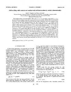
Visual inspection of the trajectories generated by MD simulations (see section 3.1) reveals signs of “hopping” motion. This is illustrated in Figure 3.1. There, in panel (a), the x-, y-, and z-components of the single particle trajectory are displayed. First, it is important to note that the particle travels only a short distance ∆r = 1.23 in a rather long time interval. This is a sign 23

of the slow dynamics observed in the supercooled regime. Furthermore, the particle travels the bulk of this distance in three distinct “hops”, i.e. within three short time intervals around t = 1050, 4550 and 9900. The positions of the particle occupied before and after the hop are clearly distinct as can be seen in panel (b) of Figure 3.1. There, 10000 positions around the hopping event at t = 4550 (time interval [4000, 5000]) are displayed in a heat map. Two clearly separated regions are visible, corresponding to before and after the jump. The inset displays the heat map for the following 10000 positions during which the particle is localized. The particle dynamics can thus be qualitatively described as a series of jumps, i.e. it travels a significant distance within very short time intervals and remains localized during the remainder of the trajectory. An algorithm has been developed to distinguish between localized motion and moves, described in detail in the following subsections 3.2.1 – 3.2.3 and in [92]. As will be discussed in chapter 4, these moves must not be directly identified with the jumps of a CTRW. Thus, an additional refinement method (see section 3.3) is applied to filter the jumps from the moves. Each detected move is characterized by the following properties: (a) The index j of the moving particle, (b) the start time of the jump tstart , (c) the end time of the jump tend , (d) the temporary equilibrium position before the jump xstart , and (e) the temporary equilibrium position after the jump xend . The jump vector is then defined as l = xend − xstart . The time of the jump is the arithmetic mean of tstart and tend , i.e. t = (tstart + tend )/2.

3.2.1

Coarse-graining in time: Time windows

A jump in the CTRW picture is infinitely fast, i.e. the particle moves from the old to the new position in a single instant. This simplification is, obviously, not physical. In the simulation this transition takes a finite time and the jump detection algorithm thus has to incorporate a coarse-graining in time. The size of these coarse-grained time windows should be as small as possible, yet large enough to fully encompass a move. For the analysis here, a time window of size ∆t = 100 was chosen, encompassing n = 1000 trajectory points. The influence of this parameter on the observed distributions is analysed in section 4.1. It is important to note that moves taking place at the edge of a time window can pass unnoticed. Thus, following the suggestion of [93], the time windows were shifted by ∆t/2 = 50 resulting in an effective sampling time of ∆t/2. Here, the time windows are denoted by W , the αth trajectory point in time window i as Wi,α and the corresponding position of monomer j as xj (Wi,α ). If move k takes place in time window i, the start and the end time of this move are identified with the midpoint of the time 24

window, i.e. tstart = tend = i · ∆t/2. Note, that tstart and tend can change k k during the refinement procedure (see section 3.3).

3.2.2

Temporary equilibrium position

In each time window, the temporary equilibrium position xmax of each particle is determined. Inspired by Figure 3.1(b) the temporary equilibrium position is defined as the position visited with the highest frequency. To this end, we first determine the average position n

1X xj (Wi ) = xj (Wi,α ) , n α=1

(3.13)

where the average is taken over all n = 1000 trajectory points in time window i. To determine the position visited with the highest frequency, the space around x is discretized into 203 cubes of volume 0.001 each. Thus, the linear dimension of the sampled region is ∆x = 2 along each coordinate axis. Then, the region containing the maximum number of trajectory points is taken as xmax (Wi ). If move k of particle j takes place in time window i, the start and end positions of this move are identified with the equilibrium positions (Wi−1 ) = xmax in the preceding and the subsequent time window, i.e. xstart j k end max and xk = xj (Wi+1 ). Note, that these positions can be modified in the refinement procedure (see section 3.3). It would also be possible to choose x as the temporary equilibrium position. We discuss this in section 4.1.

3.2.3

Move criterion

The goal is to develop a criterion that reliably distinguishes between localized motion and fast transitions. Which criterion is best suited for this task is, however, not obvious and different methods have been suggested in the literature based on the distance travelled [13, 34], on the variance [16, 38], on changes in neighboring atoms [18, 94], changes in the dihedral angle of a polymer [18, 95], and on molecule reorientation [18, 96], together with more complex methods [37, 97, 98]. To be able to assess the influence of the detection method on the results, three detection methods have been implemented. They are discussed below in detail and compared to each other in section 4.2. Variance method The first method is based on the fluctuations of a particle within a time window. As suggested in [16], the variance is used as the criterion. To this 25

end, the variance σj2 (Wi ) of particle j in time window Wi is calculated as n

σj2 (Wi ) =

1X [xj (Wi,α ) − xj (Wi )] . n α=1

(3.14)

The monomer j is labeled as moving in time window i, if σj2 (Wi ) > σc2 ,

(3.15)

where σc2 is a predefined threshold value. The following reasoning has been employed to find a physically motivated threshold value: If a particle is localized, its positions are, approximately, Gaussian distributed. For (crystalline) solids the Lindemann criterion states that melting occurs if the particle displacements about the equilibrium position reach ∼ 0.1 of the particle diameter (see, e.g., [99, 100]). Thus, one can assume that also in the supercooled and glassy states local fluctuations are roughly bounded from above by σL2 = 6rL2 = 0.054 [101] (rL ≈ 0.1). In order to label only events with a large fluctuation as moves, σc2 = 2 · σL2 = 0.108 was chosen. A detailed discussion on the influence of the detection method and the threshold value can be found in section 4.2. If not stated otherwise, the variance method has been used throughout the thesis. It has also been the method of choice in [91, 92, 102]. Displacement method Another jump detection algorithm, first suggested in [13], is based on the change of the equilibrium position of a particle. Here, the particle j is labeled as moving in time window i if |xj (Wi−1 ) − xj (Wi+1 )| > rc ,

(3.16)

where rc is an arbitrary threshold value. In reference [17], Vollmayr-Lee et al. suggest rc = 3hσi, where hσi is the average standard deviation calculated over time windows containing no move. In previous studies [13, 103, 104] a √ value of rc = 20hσi ≈ 4.47hσi was used based on visual inspection of the trajectories [103]. Distance method The third detection method is inspired by Figure 3.1 and the definition of the temporary equilibrium position, subsection 3.2.2, and has been presented in the supplementary material of [92]. If a particle is localized, all trajectory 26

points should be symmetrically distributed around its equilibrium position. Thus, the temporary equilibrium position xmax and the mean position x should coincide. In the case of a move, however, one part of the trajectory points lie in the vicinity of the equilibrium position before the move and the other part in the vicinity of the equilibrium position after the move. In this case, x is in between the two equilibrium positions, whereas xmax coincides with one of the equilibrium positions. We thus label monomer j as moving in time window i, if |xmax (Wi ) − xj (Wi )| > ∆c , j

(3.17)

where ∆c is a threshold value. The value of ∆c is discussed in section 4.2.

3.3

Refinement: From moves to jumps

A detailed analysis of the moves detected according to the procedure laid out in section 3.2 reveals that these moves do not comply with all assumptions of a CTRW (see chapter 4). This is the reason why the term “move” has been used for the detected events so far. To allow for a meaningful CTRW analysis, a refinement procedure is proposed to filter the “jumps” from the “moves”. To develop a meaningful refinement method, let us evoke the general definition of a jump: A jump is a fast transition between two distinct and uncorrelated positions. From this definition three criteria can be put forward: (1) A jump is a fast transition. Thus, the sojourn time between two jumps should be significantly larger than the time of the transition. (2) A jump connects two distinct positions. For the positions to be distinct, they need to be spatially separated. (3) The positions connected by a jump are otherwise uncorrelated. Thus, a particle should not have an increased probability to return to a previous position. We discuss these criteria in the following subsections 3.3.1 – 3.3.3. The refinement method has been presented in [92].

3.3.1

Sojourn criterion

For a move to comply with the definition of a jump, the sojourn time between the move and the previous and following move needs to be large compared to the transition time between the two minima. As the size of the time window ∆t was chosen such that it encompasses a move, the particle is required to remain localized in at least one time window between two jumps. Thus, if end moves k and k + 1 pertain to the same particle and tstart ≤ ∆t/2, k+1 − tk 0 start start end the events are replaced by a single move k with tk0 = tk , tk0 = tend k+1 , 27

end xstart = xstart and xend k k0 k0 = xk+1 . The sojourn time criterion thus requires that two jumps are separated by at least a waiting time of τmin = 100. This sets the temporal resolution of the jump detection procedure. The moves refined by this criterion are used as input for the further steps in the refinement procedure.

3.3.2

Distinct positions

As will be discussed in subsection 5.4.1, the set of moves contains a large propensity of events for which start and end position are close to each other. These events, during which the particle displays a large variance (in case of the variance method), but almost no displacement, are not recognized as jumps. Instead, these events are referred to as “loops”. Move k is labeled as a loop, if start 2 2 |xend | < rloop , (3.18) k − xk where rloop is an appropriate threshold value. Following a similar argument as for the variance method, section 3.2.3, we identify rloop = σL with the Lindemann localization length σL , i.e. the typical size of the fluctuations about equilibrium in a solid.

3.3.3

No correlations

CTRW theory assumes that the jump vectors l are completely uncorrelated. Contrary to this assumption, a large propensity of correlated moves are observed (see section 5.3). In particular, a high propensity of forward-backward moves are present [13, 16, 18, 37, 92, 94, 95, 103], i.e. events in which a particle leaves its position and then returns in the subsequent move. Moves k and k + 1 are labeled forward and backward move, if k and k + 1 pertain to the same particle and 2 |lk + lk+1 |2 < rfb , (3.19) where rfb is a predefined threshold value. In accordance with the definition of loops, subsection 3.3.2, we set rfb = σL . Furthermore, we consider the case of forward-forward correlated moves. These events can occur, if the backward move in the series forward-backward-forward remains undetected. A pair of moves k and k + 1 are labeled a forward-forward move, if k and k + 1 pertain to the same particle and |lk − lk+1 |2 < rff2 ,

(3.20)

where, again, the threshold value rff = σL is chosen. Experimental studies suggest that, in addition to this two-state switching, also three-state switching can occur [50], i.e. events in which the particle returns to its initial 28

position after two steps. For simplicity, these higher order events, which are expected to be much rarer, are not considered here.

3.4

Observables

In this section, the technical details in obtaining the observables are laid out. Subsections 3.4.1 – 3.4.5 correspond to sections 5.1 – 5.5, where the respective observables are studied in detail.

3.4.1

Waiting time distribution

The waiting time is defined as the time between two events, i.e. the time between two jumps or moves. The waiting time between the jumps or moves k and k + 1 is end τk+1 = tstart (3.21) k+1 − tk In CTRW theory, waiting times are random variables distributed according to the waiting time distribution (WTD) ψ(τ ). Note, that the term “waiting time” is also frequently used to describe the age of a glass, i.e. the time since its vitrification (see e.g. [3, 16, 103]). Here, the latter time is referred to as the age or aging time ta . To determine the WTD a histogram is constructed from a set of moves or jumps. To this end, the time is discretized into separate intervals, so-called bins, and to each bin the number of waiting times in the corresponding interval n is assigned. √ As waiting times are independent random variables, the error of n is simply n. As the WTD displays a power-law behavior over several orders of magnitude (see section 5.1), bins of varying size were used. To create a histogram with approximately nbins bins covering all times from τmin to τmax the following procedure has been applied: 1. Set the lower edge of the first bin to tle 1 = τmin . 2. Set the lower edge of the following bin to   ln[τmax ] − ln[τmin ] le le ti = ti−1 exp . nbins

(3.22)

le le 3. Round tle i such that ti − ti−1 is a multiple of ∆t/2.

4. Repeat steps 2 and 3 for all bins. The upper edge of the last bin is equal to tle nbins +1 . 29

The bins created in this way are equidistant in logarithmic time. Thus, within the power-law regime, each bin contains approximately the same number of events. To achieve a proper normalization, the count of each bin is divided by the product of the size of the corresponding time interval times th total number of waiting times used to construct the histogram. Window of observation To avoid finite size effects due to the finite length of the trajectory we introduce the time τmax and restrict the analysis to waiting times starting in the interval [0, ttrj − τmax ]. This measure ensures that waiting times τ < τmax do not display finite size effects, i.e. τmax is the maximum waiting time not influenced by the finite length of the trajectory. A discussion of finite size effects and the influence of this measure can be found in section 4.3.

3.4.2

Persistence time distribution

The persistence time τ1 is defined as the time between the start of the observation and the first jump. This time is also frequently called the “first hop time” [16], the “forward waiting time” [23], or the “forward recurrence time” [54, 67]. Here, the term persistence time was chosen in accordance with studies of dynamic facilitation [3, 4]. To obtain the persistence time distribution (PTD) ψ1 (τ1 ) from a given set of moves or jumps, a histogram was created in the same way as for the WTD.

3.4.3

Jump rate

The jump (or move) rate ν(t) is defined as the number of jumps (or moves) per unit time. To obtain the jump rate from a given set of jumps, a histogram with varying bin sizes is created as described for the WTD (see subsection 3.4.1). For each bin, one counts the number of jumps for which ti is within the corresponding time interval and multiplies the sum with 1/(tint N ), where tint is the size of the interval and N is the number of particles (or trajectories). Here, ti is the time of the ith jump.

3.4.4

Jump length distribution

The distance travelled within a move or jump is called the jump or move length. This term can refer both to the absolute distance l and to the distance 30

along one coordinate axis ξ. The jump length of jump k is defined as start lk = |lk | = |xend |, k − xk y z x ξk = eˆx · lk , ξk = eˆy · lk , ξk = eˆz · lk ,

(3.23a) (3.23b)

where eˆx , eˆy , and eˆz are the unit vectors along the x, y, and z axis. Both the distribution of the absolute distance f (l) and the distribution of distances along a coordinate axis f˜(ξ) are referred to as the jump length distribution (JLD). To obtain the JLD from a given set of jumps or moves a histogram is constructed as described for the WTD but with bins of equal size. Assuming that the distances travelled along the three spatial directions ξ x , ξ y , and ξ z are independent and identically distributed, all three contribute to the distribution f˜(ξ), which is thus a combination of f˜x (ξ x ), f˜y (ξ y ), and f˜z (ξ z ). k-jump distribution Additionally to the JLD the k-jump distribution fk is recorded, i.e. the distribution of distances after k jumps. The distribution after one jump is identical to the JLD, f1 ≡ f . For all other values of k, all pairs of jumps (i, i + k) are analysed with jumps i and i + k pertaining to the same particle, with the k-jump distance lk defined as start lk = |xend |. i+k − xi

(3.24)

The k-jump distances are used to construct a histogram similar to the one for the JLD.

3.4.5

Mean-square displacement

The mean-square displacement (MSD) g0 (t, ta ) is a common measure for the average displacement of a particle. It is a two-time correlation function and defined as N 1 X [xj (ta + t) − xj (ta )]2 , (3.25) g0 (t, ta ) = N j=1 where N is the number of particles and ta is the age of the system. In equilibrium the MSD is independent of ta , g0 (t, ta ) ≡ g0 (t), and additionally to the ensemble average in Equation (3.25) the time average was calculated to further smoothen the curve. The monomer relaxation time τ0 is defined as the time, where the MSD is equal to the monomer diameter, i.e. g0 (τ0 ) = 1 . 31

(3.26)

The monomer relaxation times for the systems under investigation have been determined according to Equation (3.26) from the MSD data obtained by Stephan Frey [83] and are listed for chains of length Nc = 4 in Table 5.2.

3.4.6

Incoherent scattering function

The self-part of the incoherent scattering function (ISF) ϕsq (t, ta ) is defined as N 1 X s exp {iq · [xj (ta + t) − x(ta )]} , (3.27) ϕq (t, ta ) = N j=1 where N is the number of particles and q is a given wave vector. The first maximum of the static structure factor |q| = q = 6.9 was chosen and the average has been taken over all vectors commensurate with the periodic boundary conditions [83]. To this end, bx =

2π , dx

by =

2π , dy

bz =

2π dz

(3.28)

were determined, where dx , dy , and dz are the linear extent of the simulation box along the respective coordinate axis. Then, the average is taken over all vectors q for which q − δq ≤ q ≤ q + δq and q · eˆx = nx bx ,

q · eˆy = ny by ,

q · eˆz = nz bz ,

(3.29)

where nx , ny , and nz are integers. As the imaginary part of the ISF will not be analysed here, Equation (3.27) can be simplified to ϕsq (t, ta )

3.5

N 1 X cos {q · [xj (ta + t) − xj (ta )]} . = N j=1

(3.30)

Internal and external time

As discussed in section 2.2, an “internal time” can be defined in the CTRW framework. To this end, a new time origin t00 is chosen for each trajectory. The internal time is then defined as t0 = t − t00 .

(3.31)

Here, two cases are of particular interest and will be discussed below: (a) The initial state with no memory, corresponding to the popular CTRW assumption of ψ1 ≡ ψ and (b) the initial state of a given non-equilibrium configuration. The implementation to transform the external to the internal time has been presented in [91]. 32

3.5.1

Initial state with no memory

To prepare the initial state with no memory, one identifies the time origin of the internal time with the time of a jump, i.e. choosing jump k of particle j one sets t00 = tk . This situation is sketched in Figure 3.2 for k = 1. It is important to note, that moves, in contrast to jumps, are not renewal events, see section 4.6. Thus, no meaningful internal time can be defined for moves. The refinement method is, however, ambiguous concerning the first jump: Assume, for example, that the first event is a backward move corresponding to a forward-move that took place before the start of the observation. In this case, the backward move is labeled as a jump. To avoid this artefact, the third jump was chosen as the new time origin for trajectories in equilibrium. For non-equilibrium trajectories, the first jump was chosen (this situation is depicted in Figure 3.2). The internal time is then defined as t0 = t − tk ,

(3.32)

where k = 3 for the equilibrium and k = 1 for the non-equilibrium trajectories. For a given particle j, the trajectory accessible in the time frame of the internal clock is ttrj − t00 . As t00 corresponds to a different point in time for each particle, the trajectories in the time frame of the internal time have varying length (see sketch in Figure 3.2). Thus, at time t0 , only trajectories can be analysed for which t00 < ttrj − t0 . If the first (or third) jump does not take place during the observation, i.e. t00 > ttrj , the trajectory can not be analysed at all. The ensemble available for ensemble averaged quantities thus shrinks for later time as less trajectories are available for the analysis. To avoid this effect, the analysis is restricted to particles for which t00 < tmax ,

(3.33)

where tmax should be chosen large enough such that sufficient trajectories are available for the analysis, but small enough such that all of these trajectories are sufficiently long. The ensemble of trajectories fulfilling the condition in Equation (3.33) remains unchanged up to time t0 = ttrj −tmax and the analysis is restricted to this time.

3.5.2

Replicate a given initial state

The internal time can be defined such that a given initial state is reproduced. This situation is sketched in Figure 3.3. Here, t00 was chosen such that the initial state of an equilibrium configuration is identical to the initial state 33

External clock:

τ1 t=0

Internal clock:

τ2 t1

t2 t3

t01 = 0

t4

t02 t03

t04

1

Figure 3.2: Sketch of the transformation from external to internal time in the case that the initial state with no memory is prepared. The horizontal lines indicate the trajectories of three particles and the ticks indicate jumps. The first jump is colored red. For the third trajectory, the jump times ti , as well as the persistence time τ1 and the first waiting time τ2 are given. This figure has been presented in [91].

34

B: A:

B τ1,j

External clock:

Internal clock:

B τ10 = τ1,j

A τ1,i

t = 0 ti,0

t0 = 0

Figure 3.3: Sketch of the transformation from external to internal time. Here, the internal time is chosen such that configuration A attains the identical PTD as configuration B. The horizontal lines indicate the trajectories of a particle from configuration B and one from configuration A. The first jump is colored red. of a non-equilibrium system. For simplicity, let us assume an equilibrium configuration A and a non-equilibrium configuration B each with a set of N A B persistence times {τ1,i } and {τ1,j }. To match the PTD of configuration A with that of configuration B, a one-to-one matching between the persistence times of configurations A and B is set up with the condition A B τ1,i ≥ τ1,j − t0a

(3.34)

for each pair of persistence times. The reasoning behind this condition will be explained later on. One of these pairs are sketched in Figure 3.3. To achieve this pairing, the following steps have been applied 1. Pick a particle j from configuration B. 2. Among the particles of configuration A, to which no corresponding B A is + t0a − τ1,j particle has been assiged yet, find particle i, for which τ1,i minimal, but larger than zero, i.e. which satisfies Equation (3.34). 3. If no particle i exists that satisfies this condition, remove particle j from the analysis. Else, assign particle j from configuration B to particle i from configuration A as its corresponding particle. 4. Repeat steps (1) – (3) until all particles of configuration B are either discarded or matched with a corresponding particle of configuration A. Once this matching is complete, the new time origin for particle i is defined as A B t00 = τ1,i − τ1,j . (3.35) The condition in Equation (3.34) can now be rationalized as follows: The observation in the time frame of the internal time starts at t00 + t0a , where 35

t0a is the age in the time frame of the internal time. Thus, the start of A B the trajectory in the external time frame is at ti,0 = τ1,i − τ1,j + t0a (see 0 sketch Figure 3.3; there ta = 0). It is obvious that ti,0 ≥ 0 from which Equation (3.34) follows directly. To gain meaningful results, Equation (3.34) requires that, on average, the persistence times of configuration A need to be larger than those of configuration B (here, let us assume t0a = 0 for simplicity). As the PTD grows broader during equilibration (see subsection 5.2.2) and hτ1 i obtains its maximum value in equilibrium, it is not possible to replicate the equilibrium dynamics using trajectories of a non-equilibrium configuration. Generally speaking, the transformation to the internal time can only be used to mimic a system farther from equilibrium than the system to which the procedure is applied. The condition in Equation (3.34) could, however, be circumvented by assuming that the particles are strongly localized before their first jump. Then, one could arbitrarily extend the trajectories by inserting intervals in which the particle is completely localized. This endeavour has, however, not been approached in this thesis.

3.6

CTRW simulations

For CTRW simulations, the stochastic process has been replicated using a random number generator, see subsection 3.6.1. If not stated otherwise, an ensemble of N = 20000 random walkers has been simulated. For each particle, its position, the number of jumps it has already performed, and the time tnext of its next jump are stored. To simulate the CTRW, the following steps have been performed 1. Place all N particles at the origin and assign to each particle the time of the next jump tnext drawn from the WTD. Furthermore, move each particle by a random distance drawn from a three dimensional Gaussian distribution with variance 6rs2 . 2. Select the particle j with the lowest time tnext for its next jump. Increase the number of jumps for particle j by one. 3. Set the time of the simulation to tnext . 4. Move particle j a random distance drawn from the jump length distribution f (l) in a random direction. This step is modified for the k-jump CTRW: Choose a new position from fk (l), where k is the number of jumps particle j has performed. 36

5. Move the particle by a random distance drawn from a three dimensional Gaussian distribution with variance 6rs2 . 6. Draw a random waiting time τ from a given waiting time distribution and set the time of the next jump of particle j to tnext + τ . 7. Repeat steps (2) – (6) until tnext is larger than the desired simulation time. Here, 6rs2 corresponds to the average fluctuations around the equilibrium position (see section 5.5). In order to obtain the single particle trajectories, the positions of all particles are stored at regular time intervals, similar as for the MD simulations.

3.6.1

Random number generation

A prerequisite for simulating a stochastic process is a solid random number generator. For the CTRW simulations random numbers were generated with the Mersenne twister [105] utilizing the implementation of the ROOT framework. The Mersenne twister is named after its very long period of 219937 − 1, which is a Mersenne prime. Random numbers in the interval (0, 1) have been generated. The methods applied to obtain random variables following a given distribution are explained below. Random numbers from a histogram In many cases it is desirable to produce random numbers distributed according to a given histogram. For example, in the CTRW simulations a random jump length is chosen from the JLD. Furthermore, random waiting times have been drawn from the WTD to confirm that the functional form used to characterize the WTD is reasonable. Let us assume a histogram consisting of nbins bins and denote with hi the value assigned to bin i. Furthermore, let us define i X si = hj , (3.36) j=1

with s0 = 0. To obtain a random variable distributed according to the histogram, first a random variable r is generated, which is uniformly distributed in (0, 1). Then, bin x is selected for which sx−1 < rsnbins < sx . Assuming a uniform distribution within bin x, the random variable
le le (3.37) rhist = tle x + r tx+1 − tx 37

is distributed according to the histogram. In Equation (3.37) tle x is the lower edge of bin x. Gaussian distribution In order to obtain Gaussian distributed random variables with mean µ and variance σ 2 the fast ACR method [106] was used as implemented in the ROOT framework. Gamma distribution Random variables distributed according to the Gamma distribution have been obtained using the algorithm suggested by Marsaglia and Tsang [107]. A lower cutoff τmin can be easily introduced by rejecting all random variables smaller then τmin . Truncated Pareto distribution In order to generate a random variables according to the truncated Pareto distribution, first two random variables r1 and r2 are generated, which are uniformly distributed in (0, 1). The first is utilized to generate a random variable rPareto distributed according to the Pareto distribution, Equation (2.24). To this end, one calculates i h − γ1 (3.38) rPareto = τ0 (1 − r1 ) − 1 . The exponential cutoff is introduced by rejecting rPareto if r2 > e−λrPareto ,

(3.39)

Random direction In the CTRW simulations, section 3.6, a random direction is chosen for the particle displacement. To this end, two random numbers r1 and r2 are generated, which are uniformly distributed in (0, 1). Then, the unit vector r in a random direction is defined as rx = sin(θ) cos(ϕ),

ry = sin(θ) sin(ϕ),

rz = cos(θ) ,

(3.40)

with θ = πr1 ,

ϕ = 2πr2 .

38

(3.41)

Chapter 4 Test of CTRW assumptions It might be an intriguing idea to identify the moves detected according to section 3.2 directly with jumps of a CTRW. On first sight, this identification might seem trivial given the striking resemblance between the single-particle trajectories of particles in a supercooled liquid and of random walkers. However, on second sight one realizes that the transition from moves in the trajectory to jumps of the CTRW is far from being trivial. The CTRW, for example, assumes an ensemble of independent random walkers, whereas the particles in a glass forming liquid are strongly interacting. Furthermore, the CTRW assumes that jumps are fully uncorrelated, contrary to other popular models for glass dynamics, such as models based on dynamic facilitation. The identification of jumps in the trajectory with jumps of a stochastic process is the crucial step laying the ground for the subsequent analysis. Thus, utmost care needs to be taken in this step. This includes a thorough analysis of the algorithm (sections 4.1 – 4.3) as well as a detailed study of the jump candidates (sections 4.4 – 4.6).

4.1

Parameter sensitivity

The algorithm to detect moves, presented in section 3.2, depends on several parameters, which need to be chosen in advance. This pertains in particular to the size of the time windows ∆t, the threshold value to detect moves σc (or rc and ∆c for the alternative move criteria) and the choice of the temporary equilibrium position. The parameters chosen for the MD simulations have already been studied in detail in [74, 83] and will not be discussed here. In order to assess the influence of the parameters, their influence on the WTD and the JLD is studied. Figure 4.1 displays these distributions using time windows of size ∆t = 50, 100, and 200, containing 500, 1000 and 2000 39

10 10 10 10 10

10

Nc = 4 T = 0.39

-5

10

~ f(ξ)

ψ(τ)

10

-3

-4

-6

∆t = 50 ∆t = 100 ∆t = 200

-7 -8

10

10

10

2

10

3

τ

10

4

10

Nc = 4 T = 0.39

-1

-2

10

-9

0

-2

5

∆t = 50 ∆t = 100 ∆t = 200

-3

0

-1

1

2

ξ

(a)

(b)

Figure 4.1: (a) WTD ψ(τ ) and (b) JLD f˜(ξ) for chains of length Nc = 4 at T = 0.39. Different symbols correspond to different sizes of the time windows used for the move detection (see section 3.2). The following sizes have been used: ∆t = 50 (blue ), 100 (red ) and 200 (green ♦).

trajectory points respectively. Both the WTD, Figure 4.1(a), and the JLD, Figure 4.1(b), display only small variations in the cutoff regime and the exponential tail, respectively. These variations remain small and do not exhibit a specific trend for the WTD, i.e. the exponential tail is neither shifted to shorter nor to longer times with decreasing (or increasing) ∆t. For the JLD, on the other hand, a clear trend can be observed with larger ∆t leading to more pronounced tails. This observation can be rationalized as follows: The time windows in which the positions before and after the jump, xstart are xend , are determined are farther apart for larger time windows. As the particles are not perfectly localized between two jumps (which will be shown in section 4.5), the jump length l tends to increase with increasing ∆t. Based on this observation it is plausible to assume that ∆t has only a small influence on the results. As the size of the time windows determine the temporal resolution, small values of ∆t are, in general, favorable. The determination of the temporary equilibrium position (see subsection 3.2.2) requires, however, sufficient statistics within a time window. As a compromise, ∆t = 100, corresponding to 1000 trajectory points within each time window, is used here. In subsection 3.2.2 xmax was identified with the temporary equilibrium position, whereas the mean position x is found more frequently in the literature [13, 17, 37, 38]. In order to assess the effect of this choice, in Figure 4.2 the WTD and JLD are displayed using xmax (red ) or x (blue l) as the temporary equilibrium position. The WTD, displayed in Figure 4.2(a), is almost completely unaffected by the choice of the temporary equilibrium position. 40

-3

10

Nc = 4 T = 0.39

10

~ f(ξ)

ψ(τ)

10 -4 10 -5 10 -6 10 -7 10 -8 10 -9 10 -10 10 -11 10 2 10

_ Mean position x Most visited position xmax

10

0

Nc = 4 T = 0.39

-1

-2

10

-3

_ Mean position x Most visited position xmax

-4

10

3

10

4

10

10 -2

5

0

-1

1

2

ξ

τ

(a)

(b)

Figure 4.2: (a) WTD and (b) JLD of the refined jumps using either x (solid blue circles) or xmax (open red squares) as the temporary equilibrium position. The distributions have been determined for chains of length Nc = 4 at T = 0.39. However, the JLD, Figure 4.2(b), differs with the JLD for x displaying less pronounced tails and an increased probability for short distances. This suggests that the time windows in which xstart and xend are determined contain part of the jump and thus x does not match with the equilibrium position. This is in line with the observation that less forward-backward moves but more loops are detected when choosing x as the temporary equilibrium position. This analysis supports the choice of xmax as the temporary equilibrium position. The influence of the threshold value for the move detection will be discussed in the following section together with the influence of the detection method.

4.2

Influence of the move detection method

For a meaningful analysis of the CTRW approach it is necessary that the relevant distributions do not depend on the specific choice of the move detection. Thus, different move criteria are studied here for a polymer melt of chain length Nc = 4 at T = 0.39. Parts of this analysis have been presented in the supplementary material of [92]. Various methods have been suggested in the literature to select moving particles. In order to assess the influence of the detection method, three candidates are discussed here: (1) The variance method, inspired by [16], (2) the displacement method as suggested in [13] and (3) the distance method as a new candidate. Details on the three detection methods can be found in subsection 3.2.3. 41

p(σ2), p(r2), p(∆2)

10 10 10

10 10

Variance method Displacement method Distance method

-1

-2

10 10

0

-3

-4 -5 -6

0

0,2

0,4

0,6

0,8

1

σ2, r2, ∆2

Figure 4.3: Distributions of the relevant parameters used for the move detection. The parameters σc2 for the variance method (blue circles), rc2 for the displacement method (green diamonds), and ∆2c for the distance method (red squares) are displayed. The vertical dashed blue line marks the parameter σc2 = 0.108 chosen for the variance method and used for the remainder of this thesis. The dash-dotted green and dotted red lines mark the corresponding parameter choices for the displacement and distance methods, respectively. The relevant parameters have been determined for all monomers in 199 (variance and distance methods) or 197 (displacement method) time windows in a system with polymers of length Nc = 4 at T = 0.39. A similar version of this Figure has been presented in the supplementary material of [92] First, the distributions of the different parameters used to detect move events are analysed, see Figure 4.3. For all three methods, an exponential decay at large values and a pronounced peak at small values can be observed, corresponding to confined motion. It is thus reasonable to choose the threshold value for the parameter at the transition between the peak and the exponential tail [37]. This consideration agrees very well with the choice σc2 = 0.108 for the variance method, as well as with the corresponding threshold values for the other detection methods (see below for how corresponding threshold values are defined). In order to compare the three detection methods, the threshold parameters are chosen such that all three methods detect approximately the same amount of moves. As discussed in section 3.2.3, the variance can be compared to the Lindemann localization length σL2 = 0.054 [101]. Thus, σc2 = σL2 , 2σL2 , and 3σL2 was chosen for the variance method and the threshold values for the other detection methods was chosen such that they detect approximately the same amount of jumps. This corresponds to rc = 0.06, 0.21, and 0.43 for the displacement method and ∆c = 0.04, 0.07, and 0.12 for the distance method. The WTD and JLD obtained using the different detection methods with the corresponding parameters are displayed in Figure 4.4. One can recognize 42

10

10 10 10 10

10

0

-4

10

-5

~ f(ξ)

ψ(τ)

10

-3

-6 -7 -8

10

10

-1

-2

10

-3

-9

10

2

10

3

10

4

10

5

-2

0

-1

1

2

ξ

τ

(a)

(b)

Figure 4.4: (a) WTD and (b) JLD for the refined jumps using different jump detection methods. The distributions are given for the variance method (symbols), the displacement method (dashed lines) and the distance method (solid lines) using the parameter sets corresponding to σc2 = 0.054 (blue), σc2 = 0.108 (red), and σc2 = 0.162 (green). The distributions have been obtained for polymers of length Nc = 4 at T = 0.39. Similar versions of these Figures have been presented in the supplementary material of [92]. that the threshold parameter has a clear influence on the obtained distributions, whereas the different detection methods overlap almost completely if they detect approximately the same amount of jumps. In general, a smaller threshold value leads to more detected jumps. Thus, it is not surprising that it also leads to a suppression of long waiting times. This pertains both to the power-law which shows a stronger decay as well as the exponential cutoff, which is shifted to shorter times. A smaller threshold value, furthermore, leads to a narrower JLD. This can be rationalized as follows: When using a larger threshold value, the monomers need to be more mobile in order to be detected. Thus, they travel farther on average. Whereas the Lindemann localization length has been chosen here as a relevant length scale to which the variance is compared, the mean standard deviation hσi, averaged over all time windows, is frequently used in the literature [16, 17]. In order to be able to compare the choice of σc2 = 0.108 used here with previous studies, the mean standard deviation was determined to hσi ≈ 0.155 for polymers with chain length Nc = 4 at T = 0.39. Thus, our choice agrees very well with the choice σc2 = (2hσi)2 = 0.0961 used in reference [16]. Furthermore, the corresponding threshold value of the displacement method rc2 = 0.21 agrees very well with the choice rc2 = (3hσi)2 = 0.216225 from reference [17]. This consideration justifies the choice of σc2 and shows that the obtained results can be directly compared with the results from the literature. Thus, if not stated otherwise, the variance method was 43

10 10

ψ(t)

10 10 10 10

-3

-4 -5 -6

full distribution not corrected corrected

-7 -8

10

τmax

-9

10

2

3

10

10

4

Ttrj

10

5

t

Figure 4.5: WTD to illustrate the effect of the finite trajectory length. The crosses display the full WTD obtained from a trajectory of length ttrj = 1.2 · 106 . For the other distributions, the length of the trajectory has been reduced to ttrj = 2·104 . The red squares display the results without correction (corresponding to τmax = 0), the blue circles the corrected result using τmax = 1 · 104 (see text for details). A system with chains of length Nc = 4 at T = 0.39 was used for the analysis. This Figure has already been presented in the supplementary material of [92]. used with σc2 = 0.108.

4.3

Finite size effects

For the analysis at hand, two types of finite size effects need to be considered: The finite system size and the finite length of the trajectories. The systems under consideration here, containing 12288 monomers, are considered large enough to not show any effects due to the finite size of the simulation box [108]. However, as the relaxation times increase strongly close to the glass transition temperature, effects due to the finite length of the trajectories need to be considered carefully. The discussion here has also been presented in the supplementary material of [92]. Finite size effects are well illustrated considering their influence on the WTD. In order to detect a waiting time, both the jump marking the start of the waiting time as well as the jump marking its end need to be within the window of observation. Consider, for example, a particle jumping at time t. Then, the subsequent waiting time τ can only be detected if τ < ttrj − t, where ttrj is the length of the trajectory. Thus, long waiting times are systematically suppressed. This is illustrated in Figure 4.5. There, the WTD determined using the full trajectory of length ttrj = 1.2 · 106 is compared to the case of a trajectory of length ttrj = 2 · 104 . If no corrections are applied, see the red squares, a strong suppression of long waiting times can be observed. It is interesting to 44

10

-4

10 10 10

10 10

-5 -6

τi-1 = 100 τi-1 = 1000 τi-1 = 10000 ψ(τ)

-7

10 10

ψ(τi | li)

ψ(τi | τi-1)

10

-3

-8

10

10 2

10

3

10

4

10

5

-5 -6

li = 0.5 li = 1.0 li = 1.5 ψ(τ)

-7

10

-9

10

-4

10

10

-3

-8 -9

10

2

10

3

τi

10

4

10

5

τi

(a)

(b)

Figure 4.6: Conditional WTDs and JLDs for unrefined moves. Panels (a) and (b) display the WTD for all moves (black ) together with the WTD for waiting times τi following a waiting time τi−1 which corresponds to the symbol at τi−1 = 100 (blue 4), τi−1 = 1000 (red ), and τi−1 = 10000 (green ♦) [Panel (a)] or jump of length li which corresponds to the symbol at li = 0.5 (blue 4), li = 1.0 (red ), and li = 1.5 (green ♦) [Panel (b)]. The correlations were tested in a melt containing polymers of length Nc = 4 at T = 0.39. Both figures have been presented in the supplementary material of [92]. note that the distribution deviates already at much shorter times from the original WTD resembling an exponential cutoff much alike the one that, in fact, takes place at later times. In order to avoid this artefact, one can restrict the analysis to waiting times which are initiated in the interval [0, tm ), with tm < ttrj . Then, the waiting time distribution is unaffected by finite size effects up to time τmax = ttrj − tm . This method corresponds to the blue circles in Figure 4.5 with τmax = 1· 104 . The corrected distribution follows the correct shape up to τmax albeit with larger fluctuations due to the reduced statistics. The technique discussed here has been applied to all WTDs throughout the thesis. Where possible, τmax has been chosen to be larger than the largest waiting time observed.

4.4

Correlations between moves and jumps

The basic assumption of a standard CTRW is that jumps are independent events, i.e. that they are uncorrelated. The results in this section have been presented in [92] and the supplementary material thereof. In order to test 45

2

2

0.6

1

0.5

0.5

0.4

-0.5

0.2

-1

0.1

0.04 0.5 ∆ξ

0.3

∆ξ

0.06

1

0

0

-1.5 -2 -2 -1.5 -1 -0.5

0.08

1.5

i+1

i+1

1.5

-0.1 0 0.5 ∆ξ

1

1.5

0

-0.5

-0.02

-1

-0.04

-1.5

-0.06

-2 -2 -1.5 -1 -0.5

2

0.02

0

i

-0.08 0 0.5 ∆ξ

1

1.5

2

i

(a)

(b)

Figure 4.7: Function ∆f˜(ξi+1 , ξi ), Equation (4.2), to highlight the correlations between subsequent moves. Panel (a) displays ∆f˜(ξi+1 , ξi ) for unrefined moves, panel (b) for refined moves, i.e. jumps. The function was evaluated for chains of length Nc = 4 at T = 0.38. Note the different scales for the color code. Both Figures have been presented in [92]. whether correlations between subsequent moves exist, the WTD for all moves is compared to the WTD restricted to waiting times τi following a short, average or long waiting time, i.e. a waiting time of length τi−1 = 100, τi−1 = 1000, or τi−1 = 10000 [see Figure 4.6(a)]. Similarly, the WTD is compared to the WTD restricted to waiting times followed by a small, medium or large jump length, i.e. a jump of length li = 0.5, li = 1.0, or li = 1.5 [see Figure 4.6(b)]. In both cases no correlations are visible. As no correlations exist before refinement, the same is bound to hold after refinement, i.e. for the jumps. In order to test whether the jump vectors of subsequent moves are correlated, a different method was adopted. For uncorrelated jump vectors it holds that f˜(ξi+1 , ξi ) = f˜(ξi+1 |ξi )f˜(ξi ) = f˜(ξi+1 )f˜(ξi ) . (4.1) Correlations can thus be identified by calculating ∆f˜(ξi+1 , ξi ) = f˜(ξi+1 , ξi ) − f˜(ξi+1 )f˜(ξi ) ,

(4.2)

where ξi+1 and ξi correspond to the same component (x, y, or z). Figure 4.7 displays this function before [Figure 4.7(a)] and after refinement [Figure 4.7(b)]. In case of uncorrelated jump lengths, ∆f˜(ξi+1 , ξi ) should be zero everywhere. For the unrefined moves, however, strong correlations 46

10 10

10

10

1

=〈l2〉k/3

~k

2

-2

10

10

-1

σk

~ fk(ξ)

10

k=2 (MD) k=2 [Eq.(4.3)] k=8 (MD) k=8 [Eq.(4.3)]

0

10

-3

0

from MD from Eq.(5)

-4 -5

-6

-4

-2

0

2

4

10

6

ξ

(a)

-1

10

0

10

1

k

10

2

(b)

Figure 4.8: (a) Distribution of displacements after k jumps fk (ξ) (k-jump distribution) determined from the MD simulation (symbols) and via Equation (4.3) (lines) for k = 2 and k = 8. (b) Variance σk2 determined from the MD simulations (blue line) and via Equation (4.3) (orange line). The dashed line gives the linear relation σk2 = hl2 ik/3, the dash-dotted line gives the slope for σk2 ∼ k for comparison. Similar versions of these Figures have been presented in [102]. can be found. The diagonal slab in Figure 4.7(a) implies an increased probability to find a length ξi+1 , if ξi ≈ −ξi+1 for the previous jump. This clear anti-correlation suggests that a high propensity of particles return to their position of origin. These events are called “forward-backward moves”. As forward-backward moves do not lead to a structural change, they must not be recognized as jumps of a CTRW and are removed in the refinement procedure (see subsection 3.3.3). Figure 4.7(b) displays the function ∆f˜(ξi+1 , ξi ) after refinement. There, the correlations are significantly reduced (see scale of the color code), but not completely removed. The reduction is, however, significant enough for the purpose here. Subsequent jumps will thus be treated as uncorrelated. The fact that subsequent jumps are uncorrelated does, however, not guarantee the absence of more complex correlations, such as correlations over several jumps. To test whether correlations over several jumps exist, the k-jump distribution fk (ξ) is calculated (see section 3.4.4). In the case of uncorrelated jumps, the k-jump distribution is given by the convolution Z fk (r) = (fk−1 ∗ f ) (r) = d3 x f (r − x)fk−1 (x) , (4.3) with f1 (ξ) ≡ f (ξ). Figure 4.8(a) displays the k-jump distribution fk (ξ) determined from the MD simulations together with fk (ξ) determined via Equation (4.3). For k = 2 both results superimpose. This confirms the result 47

presented above that two subsequent jumps can be considered uncorrelated. For k = 8, however, strong deviations are visible. Particles in the MD simulations have travelled significantly less during 8 jumps than expected for uncorrelated jumps. In order to assess this effect in more detail, Figure 4.8(b) displays the variance Z 2 (4.4) σ = ξ 2 f˜k (ξ) dξ k

as a function of k. As ξ is the x-, y, or z-coordinate of the jump vector l 2 = hl2 i/3. Furand the three components are independent, it holds that σk=1 thermore, by inserting the convolution property, Equation (4.3), into Equation (4.4) it can be readily verified that 2 σk2 = kσk=1 =k

hl2 i 3

(4.5)

for uncorrelated jumps. This result corresponds to the dashed line in Figure 4.8(b) confirming that σk2 increases linearly for uncorrelated jumps. Contrary to this expected behavior, σk2 as determined from the MD simulations displays a sub-linear increase over many jumps, turning to a linear behavior only after ∼ 100 jumps. This sub-linear increase is connected to the chain structure of the polymers and is discussed in detail in light of the MSD in section 5.5.

4.5

Localization between moves

One assumption the CTRW tacitly makes and which might easily be overlooked is the assumption that the particles are perfectly localized between two jumps. In glasses, this assumption is violated as the particles fluctuate around their temporary equilibrium positions. These fluctuations add an additional constant to the MSD, accounting for the plateau (see section 5.5). However, this interpretation assumes that the temporary equilibrium position does not change between two jumps. In order to test this assumption, the mean square displacement is calculated for the temporary equilibrium position X  max end 2 h(xmax )2 i(t) = xmax (tend (tk ) , (4.6) k + t) − x k end where the index k is calculated over all moves and t < tstart k+1 − tk . This function is displayed in Figure 4.9(a) for equilibrium configurations at different temperatures. A clear deviation from the assumption of perfectly localized

48

10

10

1

0

10

T = 0.40 T = 0.39 T = 0.38 T = 0.37

10

g0(t)

2

〈(xmax) 〉(t)

10

10

-1

-2

Ti = 2.0 Ti = 0.4 Equilibrium

-1

10 10

0

-2

10

2

10

3

10

4

10

5

10

10

6

-3

-4

10

-2

10

-1

10

0

10

1

10

2

10

3

10

4

t

t

(a)

(b)

Figure 4.9: Displacement of particles (a) between two moves or (b) before the first move. Panel (a) displays the MSD for the temporary equilibrium position xmax , Equation (4.6), in equilibrium for chains of length Nc = 4 at T = 0.37 (blue 4), 0.38 (green ♦), 0.39 (red ), and 0.40 (black ). The average in Equation (4.6) is taken over at least 1000 events. Panel (b) displays the MSD g0 (t) considering only particles which have not moved before time t. The MSD is determined for the equilibrium configuration at T = 0.37 (dashed line) and the non-equilibrium configurations (see section 3.1.6) quenched from Ti = 2.00 (red ) and 0.40 (blue ♦). The MSD is evaluated until 20% of the particles have moved. Panel (b) has been presented in [91]. particles is visible. The behavior is, furthermore, strongly temperature dependent with particles at larger temperatures travelling a significantly larger distance. Interestingly, subdiffusive motion is found between two moves. We will return to this observation in section 5.5. For the non-equilibrium configurations (see section 3.1.6) the MSD g0 (t) is displayed in Figure 4.9(b) considering only trajectories for which the time of the first move is larger than t. Again, the MSD deviates strongly from the expected behavior of a perfectly flat plateau. Furthermore, a clear dependence on the history is visible with particles quenched from a high temperature being more mobile than particles quenched from a lower temperature. The influence of this mobility between two moves is critically assessed in the light of the MSD in section 5.5 and the question whether jumps are renewal events in section 4.6.

4.6

Are jumps renewal events?

CTRW theory assumes that all jumps are independent events. Thus, the waiting times do not depend on the history of the process and, in particular, not on any previous waiting times. This assumption is not trivial in glassy 49

10

10

Ti = 2.0 Ti = 0.4 Equilibrium

-3

ν(t′)

ν(t)

10

-4

Ti = 2.0 Ti = 0.4 Equilibrium 10

-4

-5

10

2

3

10

10

4

10

5

10

10

6

-5

10

2

10

3

10

4

10

5

t′

t

(a)

(b)

Figure 4.10: Jump rate in the time frame of the external (physical) time t [panel (a)] and the internal time t0 [panel (b)]. Both panels display the equilibrium configuration at T = 0.37 (dashed line) and the non-equilibrium configurations quenched from Ti = 2.00 (red l) and 0.40 (blue ). The internal time was chosen such that the initial state with no memory is attained (see subsection 3.5.1). The horizontal dotted line indicates the equilibrium jump rate. In both cases, a polymer melt containing chains of length Nc = 4 has been considered. Both figures have been presented in [91].

systems. In fact, in other theoretical models such as kinetically constrained models and in models based on dynamic facilitation (see section 2.3 and references therein) single particle jumps are not necessarily renewal events. In order to verify that the jumps can, in fact, be treated as renewal events, the following two prediction from renewal theory has been tested: Two systems with the same PTD should display identical (ensemble averaged) dynamics. Another consequence of renewal events is that the WTD should be independent from the history of the system. This prediction has already been validated for binary mixtures [16], a similar polymer model to the one employed here [16] and amorphous silica [17] and is not considered here. In order to test the prediction above, two out-of-equilibrium configurations and one equilibrium configuration at T = 0.37 have been considered (see section 3.1.6). The results discussed here have been presented in [91]. The trajectories of all three configurations were transformed to the internal time t0 (see section 3.5). Two cases have been considered: a) All three configurations are transformed to the initial state of a fully erased memory and b) The configurations are transformed to match the initial state of one of the non-equilibrium configurations. First, let us discuss the dynamics on the coarse-grained level of the jumps. To study the dynamics on this level, the jump rate in external and internal 50

ν(t), ν(t′)

10

10

10

-3

Ti = 2.0 Ti = 0.4

-4

-5

2

10

10

3

10

4

10

5

10

6

t, t′

Figure 4.11: Jump rate ν(t) of the two non-equilibrium configurations quenched from Ti = 2.00 (red l) and 0.40 (blue ) to T = 0.37. The lines display the jump rate ν(t0 ) of the equilibrium configuration in the time frame of the internal time. The internal time has been chosen such that the initial state matches the initial state of either of the non-equilibrium configurations (see subsection 3.5.2). The data for the non-equilibrium configurations are the same as in Figure 4.10(a). In both cases, a polymer melt with chains of length Nc = 4 has been considered. This figure has been presented in [91]. time is displayed in Figure 4.10. Panel (a) displays the jump rate in external, i.e. physical time. There, the history dependence is clearly visible: The system quenched from the high initial temperature Ti = 2.00 displays a high initial jump rate corresponding to fast dynamics. The dynamics are considerably faster than those for the configuration quenched from the lower temperature Ti = 0.40. Panel (b) depicts the jump rate in the time frame of the internal time, which was chosen such that the initial state with no memory is reproduced (see subsection 3.5.1). In the time frame of the internal time the jump rates for all three configurations overlap as predicted by renewal theory. Comparing the jump rate for the internal time Figure 4.10(b) with the jump rate for the external time Figure 4.10(a) it can be noted further that the jump rate displays significantly less fluctuations in the internal time. This can be rationalized as follows: The transition of a monomer to a new position has to be considered to be part of a collective rearrangement. Thus, in general, several particles move at the same time leading to strong fluctuations. In the time frame of the internal time, however, these spatio-temporal correlations are removed and the jump rate displays a much smoother behavior. Figure 4.11 illustrates the second test case. Here, the equilibrium configuration has been transformed such that it matches the initial state of either of the non-equilibrium configurations. As expected from renewal theory, the jump rate of the equilibrium configuration superimposes with the non51

s

φq=6.9(t′, t′a)

0.8

φq=6.9(t,ta) , φq=6.9(t′,t′a)

1 4

t′a = 10

0.6 t′a = 0

0.4 0.2 0

-2

-1

0

1

2

3

4

5

10 10 10 10 10 10 10 10 10

1 0.8

ta = t′a = 100

0.6 0.4 0.2

Ti = 2.0 Ti = 0.4 Equilibrium

0 -2 -1 0 1 2 3 4 5 6 10 10 10 10 10 10 10 10 10

6

t, t′

t′

(a)

(b)

Figure 4.12: Incoherent scattering function (ISF) at |q| = 6.9, corresponding to the first peak in the static structure factor, in the time frame of the internal clock. For panel (a) the equilibrium configuration at T = 0.37 (dashed lines) and the two non-equilibrium configurations quenched from Ti = 2.00 (solid symbols) and 0.40 (open symbols) have been transformed to the state of no memory. The ISF is then evaluated at t0a = 0 (red ), 102 (blue ), 103 (green ♦), and 104 (orange 4). For panel (b) the equilibrium configuration (dashed line) and the non-equilibrium configuration quenched from Ti = 0.40 (blue ) were transformed to the initial state of the nonequilibrium configuration quenched from Ti = 2.00 (blue ). The ISF was evaluated at ta = t0a = 102 . Both figures have been presented in [91]. equilibrium configuration that has been matched. The near-perfect overlap for short t0 is trivial: At these times the jump rate is dominated by first jumps, an event which takes place at the same time for both configurations by design. However, the prediction also holds at later times. Figures 4.10(b) and 4.11 confirm that jumps may be considered as renewal events on this coarse-grained level. It does, however, not guarantee that the same holds on the microscopic level. To study the dynamics on the microscopic scale, the incoherent scattering function is displayed in Figure 4.12. In the first case, corresponding to the initial state with no memory, displayed in Figure 4.12(a), a good agreement with the predicted behavior can be found. At short times the data corresponding to the three configurations superimpose very well. At later times, t0 & 100, however, clear deviations are visible. These deviations are even stronger in the second test case, displayed in Figure 4.12(b). Here, the equilibrium configuration and the non-equilibrium configuration quenched from Ti = 0.40 have been transformed such that their initial state matches the initial state of the non-equilibrium configuration quenched from Ti = 2.00. While renewal theory states that the ISFs 52

should superimpose, it decays much stronger for the system quenched from a high temperature. To explain these deviations, let us recall that the particles are not fully localized between two moves (see section 4.5). In particular, the particles in the configuration quenched from a higher temperature are significantly more mobile before the first jump than particles in the equilibrium configuration (see Figure 4.9(b)). The deviations in Figure 4.12 thus reflect this additional mobility which is not considered on the coarse-grained level of the jumps. Now, let us return to the coarse-grained level of the jumps. The notion that these events constitute renewal events has important implications for the interpretation of glass dynamics. Consider, for example, the trap model. The notion of renewal events implies that the distribution of energies ∆E of accessible traps is constant. This excludes possible models in which structural rearrangements (i.e. jumps) lead to deeper traps. While such a model would be able to explain aging, it would imply that some sort of history dependence persists. This implies that, in the CTRW picture, aging is a purely statistical process driven only by entropy. Furthermore, the ability to detect renewal events could have important implications for the study of mechanical rejuvenation: During aging the dynamics in glassy materials slow down over time. The dynamics do, however, increase when physical forces act on the glass, seemingly bringing the glass to a “younger” state. This observation is called mechanical rejuvenation [44, 109]. However, in this concept the term age remains a rather vague notion. Given the existence of renewal events, the ideal age zero could be associated with the state of no memory and dynamic properties could be compared to the evolution from this ideal initial state. Activated dynamics in glassy materials under external forces have been studied based on the CTRW framework [35, 36] demonstrating that both the WTD as well as the PTD are influenced by the external forces. A study of the activated dynamics after the external force is turned off, however, seems to be missing from the literature. Furthermore, it would be of high interest to test, whether the renewal holds not only for supercooled liquids but also in the glassy state.

53

54

Chapter 5 Analysis of the observables After verification in chapter 4 that the jumps detected by the algorithm described in chapter 3 can be, to good approximation, considered as jumps of a CTRW, the corresponding observables are analysed and discussed in this chapter.

5.1

Waiting time distribution

The waiting time distribution (WTD) is the central distribution governing the time-development of the CTRW. It is based on the fundamental property of a CTRW that all waiting times are identically distributed random variables, independent from the history of the system. This is equivalent to the statement that jumps are renewal events, which was demonstrated in section 4.6. The WTD has been determined from the MD simulations according to subsection 3.4.1 and is studied here in detail.

5.1.1

Effect of refinement

First, let us discuss the influence of the refinement method proposed in section 3.3. The effect of refinement on the WTD has also been discussed in [92]. To this end, the WTDs before and after refinement are displayed in Figure 5.1 together with the distribution of times between a forward and the corresponding backward move. First, it is important to note that all three distributions follow the same qualitative shape: A power-law decay at short times up to approximately the monomer relaxation time, where it crosses over to a stronger, exponential-like cutoff. This shape resembles strongly the Gamma distribution (see subsection 2.5.1) for a power-law exponent γ < 1 or an exponentially truncated stable distribution (see subsection 2.5.3) for 55

10 10

ψ(τ)

10 10 10 10

τ0

-5 -6 -7

moves jumps forward-backward moves

-8

10 10

-3

-4

-9

-10

10

2

10

3

10

4

5

10

10

6

τ

Figure 5.1: WTD for unrefined moves (green ), refined moves, i.e. jumps, (red ) and forward-backward moves (blue X). The distribution for forwardbackward moves is the distribution of times between a forward and the corresponding backward move. All distributions have been recorded for a polymer melt with chainlength Nc = 4 at T = 0.37. The lines are power-law fits to the data, ψ(τ ) ∼ τ −γ . The fit results are γ = 0.94 (jumps, solid line), γ = 1.16 (moves, dashed line) and γ = 1.5 (forward-backward moves, dash-dotted line). The vertical dotted line marks the monomer relaxation time τ0 (see subsection 3.4.5). The figure has been published in [92]. γ > 1. The second important observation that can be drawn from Figure 5.1 is that all three distributions differ strongly. This observation underlines the fact that the refinement procedure is not a mere philosophical discussion, but has a clear influence on the measured distributions. The central conclusion that can be drawn from Figure 5.1 is that the distribution of times between a forward and the corresponding backward move (blue X) displays a much steeper decay than the distribution between two moves of any type (green

). Fitting the power-law regime to ψ(τ ) ∼ τ −γ yields γ = 1.5 for the forward-backward moves and γ = 1.16 for all moves. This result is not surprising when we recall that the dynamics can be interpreted as a particle traversing a complex energy landscape. During this process, the particle might encounter a double-well, i.e. two minima which are separated by a potential barrier much smaller than the average potential barrier. In such a double well, the smaller the barrier, the more often the particle crosses the barrier. This influences the distribution twofold: First, a smaller barrier leads to shorter waiting times in either of the wells and second it leads to more barrier crossings before the particle leaves the double well and thus more detected waiting times. Both aspects strongly enhance the detection of short waiting times leading to a much steeper decay. Note that this situation differs strongly from the trap model discussed 56

in section 2.1. There, one assumes that the potential barriers separating a potential well from its neighbors all have the same height. Thus, all potential wells are visited with the same probability (and thus with the same frequency). Clearly, this assumption is violated for the forward-backward moves, a strong argument in favor of the refinement procedure which filters out these moves. On the other hand, a detailed analysis of these double-well structures could reveal properties of the underlying complex energy landscape. To achieve this goal, long series of forward-backward moves would need to be recorded in order to gain sufficient statistics. Within the temperature range studied here, however, the series of forward-backward moves contained maximum 23 moves. As the fraction of forward-backward moves increases with decreasing temperature (see section 5.3) this could, however, be achieved at lower T . Fitting the power-law decay for the refined moves, i.e. the jumps, an exponent of γ = 0.94 is found. While this value seems to be close to the exponent for all moves, γ = 1.16, the influence of the refinement procedure may not be underestimated. It is, in particular, important to note that γ < 1 for the jumps, excluding the standard version of the popular trap model as a possible microscopic model. The strong influence of forward-backward moves instead suggests that a barrier model might be more appropriate. The influence of the refinement method, furthermore, offers an explanation for the large range of exponents reported in the literature. For instance, no refinement procedure has been adopted in Refs. [16, 33, 35, 36], where exponents in the range of 1.1 < γ < 1.6 have been reported. On the other hand, some aspects of refinement have been incorporated in Refs. [13, 17] and exponents in the range of 0.3 < γ . 1.0 have been reported. Furthermore, an exponent of γ = 2 has been found in an analysis including only forward-backward moves [50].

5.1.2

Temperature and chain-length dependence

After having discussed the general shape of the WTD in the previous subsection 5.1.1, let us now turn to the temperature and chain length dependence of this distribution. The temperature and chain length dependence has also been presented in [102]. To this end, the WTDs for chains of length Nc = 4 and Nc = 32 at various temperatures are displayed in Figure 5.2. First, it is important to notice that the general shape, i.e. a power-law decay at short and a stronger cutoff at late times, remains unchanged. Panel (b) furthermore shows that the cutoff can be well described by an exponential decay. However, other functional forms can not be ruled out. For example, a second, stronger power law has been suggested in studies of transitions in the 57

~t

10 10 10 10 10

Nc = 4

T = 0.37 T = 0.38 T = 0.39 T = 0.40

-4 -5

~t

-1

10 10

ψ(t)

ψ(t)

10

-1/2

-3

-6 -7

10 10

-8

10

10

10

-9

10

2

10

3

4

10

10

5

10

Nc = 32

τ0

T = 0.42 T = 0.43 T = 0.44

τ0

-4 -5 -6 -7

~e

~e

-at/τ0

-at/τ0

-8

10

6

-3

-9

10

2

10

3

4

10

t

10

5

10

6

t

(a)

(b)

Figure 5.2: WTDs for chains of length Nc = 4 (panel a) and Nc = 32 (panel b). In panel (a) the WTDs are displayed at temperatures T = 0.37 (orange ∗), 0.38 (blue ), 0.39 (green X) and 0.40 (red ). The solid lines are the slopes for power-law decays with exponent −0.5 and −1.0 for comparison. In panel (b) the WTDs are displayed at T = 0.42 (blue ), 0.43 (green X) and 0.44 (red ). The dotted lines mark the value of the monomer relaxation time τ0 (see subsection 3.4.5) and the solid lines are exponential fits to the tails. Similar versions of these figures have been presented in [102].

potential energy landscape [31]. As the exact shape of the cutoff does not have a strong influence on the overall dynamics we can assume an exponential shape for simplicity. Thus, since the exponent of the power-law decay is within the interval −1.0 < γ < 0, the WTD can be described as a Gamma distribution (see subsection 2.5.1), fully defined by the shape parameter α and the rate parameter λ. Figure 5.2 reveals that both parameters depend on temperature and chain length. The Gamma distribution has been fitted to all WTDs. The parameters α and λ obtained by this fitting procedure are listed in Table 5.1. Standard mode-coupling theory (MCT) suggests that dynamic observables superimpose when scaled by a relevant time scale such as the monomer relaxation time τ0 [47]. This data collapse, known as the time-temperature superposition principle (TTSP), is often employed to study dynamics in polymer melts [110, 111] and glasses [42, 46, 47]. For the system at hand, however, MCT is only valid for temperatures above T = 0.40 for Nc = 4, T = 0.43 for Nc = 16 and T = 0.44 for Nc = 32 [83]. TTSP is thus expected to become violated in the temperature range studied here. This can be seen in Figure 5.3, where the WTD is displayed as a function of the rescaled time t/τ0 . While the exponential cutoffs superimpose for the rescaled time, strong deviations 58

T α λ

0.37 0.12 4.9 · 10−6

T α λ

T α λ

Nc = 4 0.38 0.39 0.22 0.30 −5 1.9 · 10 6.0 · 10−5

0.40 0.42 1.9 · 10−4

0.41 0.27 3.6 · 10−5

Nc = 16 0.42 0.35 9.8 · 10−5

0.43 0.44 2.4 · 10−4

0.42 0.32 6.9 · 10−5

Nc = 32 0.43 0.39 1.6 · 10−4

0.44 0.48 3.5 · 10−4

Table 5.1: Fit results for the shape parameter α and the rate parameter λ obtained by least-square fit of the Gamma distribution, Equation (2.20), to the WTDs. -1 -2

-5 -6 -7

ln[t ψ(t)]

ln[t ψ(t)]

-3 -4

Nc = 4 T = 0.37 T = 0.38 T = 0.39 T = 0.40 Eq. (2.8), α = 0.5 Eq. (2.8), α = 0

-8 -8 -7 -6 -5 -4 -3 -2 -1 0 1 2 3

ln[t/τ0]

0 T=0.4 (Nc=4) -1 -2 -3 T=0.43 (Nc=16) -4 -5 Nc = 32 T = 0.42 -6 T = 0.43 -7 T = 0.44 -8 -8 -7 -6 -5 -4 -3 -2 -1 0 1 2 3

ln[t/τ0]

(a)

(b)

Figure 5.3: Plot of ln[tψ(t)] versus ln[t/τ0 ] for chains of length Nc = 4 (a) and Nc = 32 (b). The data and representations of the WTDs are identical to Figure 5.2. Panel (a) includes furthermore the Gamma distributions with shape parameter α = 0.5 (solid line) and α = 0.0 (dashed line). Panel (b) includes further the WTD for chains of length Nc = 4 at T = 0.43 and of length Nc = 16 at T = 0.40. Both figures have been presented in [102]. are visible in the power-law regime. These deviations are connected with the temperature dependence of the shape parameter α. This parameter is close to α = 0.5 at high temperatures and approaches α = 0.0 at low tempera59

tures. In fact, these limiting cases very well describe the distributions for Nc = 4 at T = 0.40 and T = 0.37, respectively (see Figure 5.3(a)). At higher temperatures, i.e. in the regime where the TTSP is expected to hold, we find α ≈ 0.5 for all chain lengths (see Figure 5.3(b)). Furthermore, the results indicate that α tends toward 0 with decreasing temperature. As it is already close to this limiting value it is plausible to assume that α will not change strongly and that TTSP again holds at lower temperatures. The physical interpretation of this limiting value will be discussed in section 5.3. In Figure 5.3 the data is presented in the form of ln[tψ(t)] versus t/τ0 as suggested in reference [112]. This presentation helps to test whether the WTD follows the distribution "  2 # ln(τ /τ0 ) 1 , (5.1) ψ(τ ) = √ exp − ε τ πε where τ0 = ν0−1 is the characteristic trap lifetime and ε = E0 /kB T with E0 being a characteristic energy scale. This distribution follows from the trap model with a Gaussian distribution for the depths of the potential wells [112], i.e. for  ¯ 2 1 (∆E − E) p(∆E) = √ exp − . (5.2) E02 πE0 In the representation chosen for Figure 5.3 distributions of this type take the shape of a parabola. The WTDs studied here, however, do not fulfill this prediction, but instead are better described by a Gamma distribution, Equation (2.20). Now, let us take a closer look at the rate parameter λ. With decreasing temperature the rate also decreases, shifting the cutoff to later times. Thus, the power-law regime extends to later times for lower temperatures. Furthermore, we find that the inverse of the rate parameter, λ−1 , is approximately proportional to the monomer relaxation time τ0 with λτ0 ≈ 0.6. This observation can be rationalized alluding to the trap model (see section 2.1). In this model, the power-law behavior arises from the fact that the particle is trapped in a potential well of a random, but constant energy depth. In glasses, this potential well reflects the confinement of the particle by its neighbors. On short time scales it is reasonable to assume that the depth of the potential well is constant in time. On the time scale of the monomer relaxation time, however, rearrangements in the environment of the particle can influence the potential well. Thus, it is plausible to attribute to it an average depth on time scales longer than the monomer relaxation time, leading to an exponential behavior of the WTD. Note, however, that these considerations are purely speculative. It is, in particular, important to keep 60

in mind that the (standard) trap model leads to a stronger power-law decay than observed here.

5.1.3

Mean waiting time

The mean waiting time hτ i is defined as Z ∞ hτ i = τ ψ(τ ) dτ .

(5.3)

0

The cutoff in the WTD guarantees that the integral in Equation (5.3) takes a finite value. In the case of the Gamma distribution, Equation (2.20), the mean waiting time is α (5.4) hτ i = . λ Thus, hτ i is expected to vanish for α → 0, i.e. with decreasing temperature. It is important to note, however, that due to the finite resolution of the numerical analysis two jump events need to be separated by at least τmin = 100 (see subsection 3.3.1). In this case, instead of Equation (5.3), the effective mean waiting time is obtained as Z ∞ τ ψ ∗ (τ ) dτ . (5.5) hτ ieff = τmin

Introducing the finite resolution, the Gamma distribution takes the form ( λα tα−1 e−λt for t > τmin ∗ Γ(α,λτmin ) ψ (t) = fλ,α,τmin (t) = (5.6) 0 else, where

Z

∞

Γ(s, x) =

ts−1 e−t dt

(5.7)

x

is the upper incomplete Gamma function. The effective mean waiting thus takes the form hτ ieff =

Γ(α + 1, λτmin ) (λτmin )α e−λτmin = hτ i + . λΓ(α, λτmin ) λΓ(α, λτmin )

(5.8)

Thus, even if α vanishes, the observed mean waiting time remains finite. Comparing Equation (5.8) with Equation (5.4), it can be found that the influence of α is less strong on the effective mean waiting time. This is not surprising as a decreasing value of α is expected to lead to a strong increase in extremely short waiting times, which are, however, not detected due to the 61

T hτ ieff observed hτ1 i observed τ0 hτ ieff from Equation (5.8) hτ i from Equation (5.4) hτ1 ieff from Equation (5.19) hτ1 i from Equation (5.18)

0.37 4.5 · 104 1.0 · 105 1.2 · 105 4.3 · 104 2.4 · 104 1.1 · 105 1.1 · 105

Nc 0.38 1.6 · 104 2.2 · 104 3.2 · 104 1.6 · 104 1.1 · 104 3.2 · 104 3.2 · 104

=4 0.39 7.6 · 103 6.9 · 103 1.0 · 104 6.6 · 103 5.0 · 103 1.1 · 104 1.1 · 104

T 0.41 hτ ieff observed 1.0 · 104 hτ1 ieff observed 1.6 · 104

Nc = 16 0.42 0.43 3 4.7 · 10 2.4 · 103 6.3 · 103 3.0 · 103

T 0.42 hτ ieff observed 6.1 · 103 hτ1 ieff observed 9.1 · 103

Nc = 32 0.43 0.44 3 3.2 · 10 1.7 · 103 4.6 · 103 2.0 · 103

0.40 3.1 · 103 2.3 · 103 3.9 · 103 2.8 · 103 2.2 · 103 3.7 · 103 3.7 · 103

Table 5.2: Effective mean waiting times hτ ieff and effective mean persistence time hτ1 ieff as observed in the jump-analysis of the MD trajectories. For Nc = 4 also the monomer relaxation time τ0 (see subsection 3.4.5) and the analytic results for the mean waiting time, Equation (5.8) and Equation (5.4), and for the mean persistence time, Equation (5.19) and Equation (5.18), are listed. For the analytic results, the parameters from Table 5.1 were used.

finite resolution. Thus, the effective mean waiting time is expected to depend more strongly on λ and to increase with decreasing temperature. This can be seen in Table 5.2 where all mean waiting times are listed. For Nc = 4 also the results of Equation (5.8) and Equation (5.4) are given using the parameters from Table 5.1. It can be found that the mean waiting time according to Equation (5.4) increases slower than the observed mean waiting time. This observation highlights the fact that the finite resolution, and the finite time necessary for a rearrangement, becomes relevant at low temperatures. The method applied here does, however, not allow for a better resolution. Different methods based on an analysis of the potential energy landscape [29] or transition path sampling [113, 114] might be better suited to answer the question how long the transitions take and thus determine the value of τmin independent from the choice of time windows. 62

Nc = 4

ψ1(τ1)

10 10 10 10 10

T = 0.37 T = 0.38 T = 0.39 T = 0.40

-4 -5 -6 -7 -8

10

2

10

3

10

4

10

5

10

6

τ1

Figure 5.4: Persistence time distribution ψ1 (τ1 ) for chains of length Nc = 4 at temperatures T = 0.37 (orange ∗), 0.38 (blue ), 0.39 (green X) and 0.40 (red ). Error bars are only given for T = 0.40. In all other cases the errors are of the same order of magnitude.

5.2

Persistence time distribution

Whereas the waiting time is defined as the time between two jumps, the persistence time is defined as the time between the start of the observation and the first jump. The distributions of these two observables differ significantly. Here, the term “persistence time” was chosen following the nomenclature used for kinetically constrained models [10, 115]. There, the “persistence time” is contrasted to the “exchange time” which corresponds to the waiting time in the analysis at hand. In the field of stochastic processes the persistence time is more commonly called the “first waiting time” [56] or “forward recurrence time” [54, 67]. The PTD is of particular interest as it, in contrast to the WTD, displays aging, i.e. it is dependent on the history of the system.

5.2.1

Equilibrium case

Before turning to the history dependence of the PTD, however, let us first study its equilibrium properties. Parts of this analysis have been published in [102]. To this end, the PTD for chains of length Nc = 4 at various temperatures is displayed in Figure 5.4. It is important to note, that the shape of the PTD differs strongly from the WTD (see Figure 5.1). In particular, the WTD displays a much stronger decay at short times whereas the PTD is almost flat in this regime at low temperatures. The strong decay of the WTD corresponds to a high probability of very short waiting times, whereas the shape of the PTD suggests that long persistence times play a dominant role. CTRW theory predicts that in equilibrium the PTD ψ1 is closely related 63

to the WTD ψ via the equation [23, 66, 67] Z ∞ 1 ψ1 (t) = ψ(t0 ) dt0 . hτ i t

(5.9)

This relation is readily derived using the following argument. In equilibrium the dynamics obey time symmetry. Inverting the direction of time, the probability for the persistence time t becomes the probability that the last jump took place a time t ago, which is equivalent to the probability of a waiting time larger than t. This probability can be expressed as Z ∞ ψ1 (t) ∼ ψ(t0 ) dt0 . (5.10) t

The prefactor in Equation (5.10) then follows from the fact that the PTD needs to be normalized. In the case of a Gamma distribution (Equation (2.20)), the PTD takes the form λ Γ(α, λt) , (5.11) ψ1 (t) = α Γ(α) where Γ(x) is the Gamma function (Equation (2.17)) and Γ(s, x) the upper incomplete Gamma function (Equation (5.7)). Equation (5.11) suggests that the PTD seizes to be normalizable for α = 0. This is due to the fact that the mean waiting time vanishes. As discussed in subsection 5.1.3, however, the finite resolution guarantees that hτ i stays finite even for α = 0. Taking this finite resolution into account, the PTD takes the form  λΓ(α, λt)   for t > τmin ,  Γ(α + 1, λτmin ) (5.12) ψ1 (t) = 1    else . hτ ieff In the two limiting cases, it can be found that √ ψ1 (t) ∼ erfc( λt) for α = 0.5 , where

2 erfc(x) = √ π

Z

∞

2

e−t dt

(5.13)

(5.14)

x

is the complementary error function [69] and ψ1 (t) = −λeλτmin Ei(−λt) for α = 0 , 64

(5.15)

10 10 10 10

-1

〈τ〉eff

-4

T = 0.39 Nc = 4

10

~ erfc[(λt)1/2]

-5 -6

ψ1(t)

ψ1(t)

10

τ0 MD simulation CTRW simulation calculated from ψ(t)

-7

10 10

-8

10

10

10 2

10

3

10

4

10

5

~ -Ei[-λt]

-4

T = 0.37 Nc = 4

-1

〈τ〉eff

τ0

-5 -6

MD simulation CTRW simulation calculated from ψ(t)

-7 -8

10

2

10

3

10

4

10

5

10

6

t

t

(a)

(b)

Figure 5.5: PTD for T = 0.39 and T = 0.37 with analytic solutions given in Equation (5.13) and Equation (5.15). The MD data is identical to the data presented in Figure 5.4. The figure in panel (a) has been published in [102]. where

Z

∞

Ei(x) = − −x

e−t dt t

(5.16)

is the exponential integral [69]. In order to compare the analytic result to the MD simulations, the PTD for chains of length Nc = 4 at T = 0.39 and 0.37 is displayed in Figure 5.5. There, the PTD has been obtained in three ways. First, the PTD has been directly determined from the MD simulations (blue X). These data are identical to the data displayed in Figure 5.4. The second method is a CTRW simulation (red , see section 3.6) of 50000 particles using the WTD obtained from the MD simulations. The CTRW has been simulated until equilibrium was reached, i.e. for a time t = 2.5 · 106 for T = 0.37 and t = 5 · 105 for T = 0.39. The PTD distribution is then determined as the distribution of times until the next jump. The third method used to determine the PTD is based on Equation (5.9), where the WTD obtained from MD simulations is integrated numerically. Figure 5.5 shows that the PTDs for all three methods overlap. This consistency check is another argument that the single-particle dynamics can be described as a CTRW. Furthermore, it demonstrates that, in equilibrium, the PTD can be obtained directly from the WTD. This plays an important role for the CTRW simulations as it reduces the number of distributions needed as input to the CTRW simulations by one. In previous studies, the PTD has been determined from the MD simulations [16] or from the incoherent scattering function [33] prior to be used in CTRW simulations. In addition to the PTD determined from the simulations, the analytic result for the limiting cases α = 0.5 and α = 0 is displayed for T = 0.39 and T = 0.37, respectively. These limiting cases describe very well the PTD at 65

10

10 10 10 10

Nc = 4

ta = 0

-4

10

-5

10

-6 -7

ta = 10

ψ1(t′,t′a)

ψ1(t,ta)

10

-3

5

10 10

-5

-8

-9

10 2

10

3

10

4

10

5

10

6

ta = 10

-7

10

10

5

-6

-8

10

Nc = 4

ta = 0

-4

-9

10

2

10

3

10

4

10

5

10

6

t′

t

(a)

(b)

Figure 5.6: PTD for two non-equilbrium configurations of chains of length Nc = 4 quenched from Ti = 0.40 (open symbols) and 2.00 (solid symbols) to T = 0.37. Panel (b) further displays the PTD for the equilibrium configuration at T = 0.37 (dashed lines). The distributions are displayed at three different aging times ta = 0 (red ), 103 (green ♦) and 105 (cyan O). Panel (a) displays the PTD in the time frame of the external time t, panel (b) in the time frame of the internal time t0 , where the initial state of no memory was attained (see section 3.5). Panel (b) also includes the WTD at T = 0.37 (solid line). high and low temperatures. This demonstrates one of the strengths of the CTRW description of glass dynamics: Based on a simple functional form for the WTD analytic results can be obtained for many other observables.

5.2.2

Non-equilibrium case

Both theory [54, 56] and previous studies [16] suggest that the PTD displays a strong history dependence. In other words, it depends on the system preparation as well as on the age of the system, i.e. the time elapsed since the system was prepared. In order to study the history dependence, the PTD is displayed in Figure 5.6 for two configurations, prepared using different quench protocols (see subsection 3.1.6 for details). The left panel of Figure 5.6 displays the PTD as observed in external time. As it would be expected, the PTDs directly after the quench, i.e. at ta = 0, differ for the two quench protocols. The difference is, however, very small and occurs only at short times. Already after the system has been aged for ta = 103 , a time two orders of magnitude shorter than the equilibration time, the PTDs for the two different configurations superimpose. This observation is surprising, as the jump rates superimpose only for times t & 104 (see Figure 4.10(a)). The right panel of Figure 5.6 displays the PTD in the time frame of the 66

internal time t0 (see section 2.2 for the internal time and section 3.5 how the transition from external to internal time is performed). As expected, no history dependence can be observed in this time frame. This agrees with the identical observation for the jump rate in section 4.6 and serves as an additional argument that the jumps may be treated as renewal events. The internal time is chosen such that ψ1 (t) ≡ ψ(t), corresponding to the initial state of no memory. In order to verify this relation, the WTD is included in Figure 5.6(b). A very good agreement between ψ1 (t, ta = 0) and ψ(t) can be found with only a small deviation at very short times. On aging, the PTD changes its shape. In particular, the probability of short persistence times decreases considerably. Correspondingly, the probability for long persistence times increases. Thus, during aging the mean persistence time increases leading effectively to slower dynamics on short time scales.

5.2.3

Mean persistence time

If the second moment of the WTD exists, the equilibrium value of the mean persistence time hτ1 i can be calculated as [28] hτ 2 i . hτ1 i = 2hτ i

(5.17)

This relation follows directly from Equation (5.9). As hτ 2 i ≥ hτ i2 , it holds that hτ1 i/hτ i ≥ 1/2. In the case of the Gamma distribution, one finds hτ1 i =

α+1 . 2λ

(5.18)

This relation suggests that the ratio hτ1 i/hτ i diverges as α approaches 0, i.e. as the temperature is decreased. However, similar to the considerations concerning the mean waiting time (see subsection 5.1.3) it is necessary to take the finite resolution into account. In this case, the mean persistence time takes the value hτ1 ieff

1 Γ(α + 2, λτmin ) (λτmin )α+1 e−λτmin = = hτ1 i + . 2 λΓ(α + 1, λτmin ) 2λΓ(α + 1, λτmin )

(5.19)

The values of the mean persistence times for all configurations considered in this thesis are listed in Table 5.2. For configurations of chain length Nc = 4 also the results of Equation (5.18) and Equation (5.19) are given. It is interesting to note that, contrary to the case for the mean waiting time, both equations yield the same results within the certainty of the parameters used. This is, however, not surprising and can be rationalized as follows. The 67

2,5

〈τ1〉eff/〈τ〉eff τ0/〈τ〉eff

2,0

1,5

1,0

1/Tc 0,5 2,5

2,6

2,7

1/T

Figure 5.7: Ratio of the mean persistence time to the mean waiting time hτ1 ieff /hτ ieff as a function of the inverse temperature observed in a system containing chains of length Nc = 4. Additionally, the ratio τ0 /hτ ieff is depicted, where τ0 is the monomer relaxation time (see subsection 3.4.5). The vertical dotted line indicates the value of 1/Tc (Tc = 0.383 [83]). The horizontal dashed line gives the minimum value for hτ1 ieff /hτ ieff . A similar version of this figure has been presented in [92]. mean persistence time is proportional to the second moment of the WTD. Thus, the short time behavior of the WTD has a much smaller influence on the mean persistence time than on the mean waiting time. Therefore, removing the extremely short waiting times from the analysis hardly affects the mean persistence time. Comparing the values of the mean waiting time hτ ieff to the mean persistence time hτ1 ieff , it can be realized that hτ ieff and hτ1 ieff are close at high temperatures, i.e. for T > Tc . On cooling through Tc , however, hτ1 ieff increases much more strongly than hτ ieff . This can be seen in Figure 5.7. This discrepancy can be interpreted as the violation of the Stokes-Einstein relation [3, 4, 116]. The Stokes-Einstein relation describes the observation that the diffusion coefficient D is inversely proportional to the viscosity η [117] D=

kB T , 6πηr

(5.20)

where r is the radius of the diffusing particle. Equation (5.20) describes the intimate connection of the dynamics on the short time scales, determining the viscosity, with the dynamics on the long time scales, governing the diffusion coefficient. This relation is, however, violated in glass forming liquids. The violation of the Stokes-Einstein relation can be interpreted in terms of two relevant time scales: The time scale of the viscosity corresponds to the time scale until all particles have rearranged at least once, which is related to the mean persistence time. On the other hand, the time scale of diffusion 68

corresponds to the average time between two rearrangements, which corresponds to the mean waiting time [10, 115]. Thus, a splitting of these two time scales leads directly to a violation of the Stokes-Einstein relation.

5.3

Jump rate

The jump rate ν(t, ta ) is defined as the probability of a jump in a given time interval. Multiplied with the number of particles or random walkers the jump rate thus gives the (average) number of jumps per unit time. As a high frequency of jumps corresponds to large displacements, the jump rate can be used to distinguish between “slow” and “fast” dynamics. The jump rate in equilibrium has also been discussed in [92], the non-equilibrium jump rate has been discussed in [118].

5.3.1

Equilibrium case

In equilibrium a constant jump rate is observed, i.e. ν(t, ta ) ≡ ν = const. In Appendix A it is shown, how the constant jump rate arises from CTRW theory assuming a system in equilibrium. As the jump rate is constant, it can be determined as the total number of jumps (or moves) divided by the length of the trajectory, i.e. νx =

Nx (T ) , nt tm

(5.21)

where Nx is the total number of moves of a given type, nt = 12288 the number of analysed trajectories, and tm the length of the trajectories. The jump rate has been analysed for moves of any type (also called the move rate). Furthermore, the moves have been distinguished into loops, forwardbackward moves and jumps. It is important to note that the number of loops, forward-backward moves, and jumps sum up to the total number of moves, i.e. Nloop + Nfb + Njump = Nmove . Thus, also the relative frequency of a given type can be calculated as νx . (5.22) ωx = νmove Both the absolute and relative frequencies for the move types considered here are displayed in Figure 5.8 for chains of length Nc = 4. First, it is interesting to note that the absolute frequency of moves is very small. Taking into account that the size of one time window is ∆t = 100 (see subsection 3.2.1), one finds that on average between 3.75% (at T = 0.40) and 0.18% (at T = 0.36) of the monomers move per time window, confirming the 69

1.0

moves jumps

-4

10

ωx(T)

νx(T)

1/Tc

forward-backward moves loops

0.5

-5

10

1/Tc

2,5

2,55

2,6

2,65

2,7

0.0

2,75

2,5

2,6

2,7

1/T

1/T

(a)

(b)

Figure 5.8: Absolute (panel a) and relative (panel b) frequency of moves of different types as a function of the inverse temperature for chains of length Nc = 4. The vertical dashed line marks the value of 1/Tc (Tc = 0.383 [83]). The lines in panel (a) display an Arrhenius fit (Equation (5.23)) to νmove (T ) (solid line) and a Vogel-Fulcher-Tammann fit (Equation (5.24)) to νjump (T ) (dashed line). Both figures have been presented in [92]. premise that moves are rare events. Second, one can notice that the absolute frequency decreases with decreasing temperature for all move types. This corresponds the fact that the dynamics are significantly slower at lower temperatures. However, the decrease in the absolute frequency is different for the different move types. The rate for all moves follows closely an Arrhenius behavior [41]   Ca , (5.23) ν(T ) = ν0 exp − kB T with Ca being a temperature independent activation energy. A least-square fit to νmove yields Ca ≈ 28.8kB Tc and 1/ν0 ≈ 2.9 · 10−9 τLJ . The activation energy obtained in this way is rather large but still in the range typically found in experimental studies of flexible polymers (see Table II in [43] and references therein). For various other glass formers activation energies around 10kB Tg (≈ 8kB Tc [43]) are reported [49, 119, 120]. While the activation energy attains a reasonable value, the prefactor is several orders of magnitude smaller than expected. The time scale for the prefactor corresponds approximately to 1/ν0 ∼ 10−20 s (as τLJ ≈ 10−11 s [108]) which is far off from an expected value on the order of 10−14 s ≈ 10−3 τLJ [43, 121]. A strong deviation from the expected order of magnitude, as observed here, can occur if the temperature range over which the data is fitted is too small [121]. Thus, the fit results need to be treated with care. In order to obtain more reliable values, the analysis would need to be extended to lower temperatures. 70

While the rate for all moves decreases Arrhenius-like, it decreases much stronger for jumps. The reason for this stronger decrease is that the relative frequency of loops and forward-backward moves increases with decreasing temperature (see panel (b) in Figure 5.8). Whereas at T = 0.40 jumps constitute 87% of all moves this value decreases to approximately one third at T = 0.36 and is projected to decrease further at lower temperatures. Accordingly, the propensity of correlated motion, i.e. loops and forward-backward moves, increases strongly with decreasing temperature. This observation suggests that at lower temperatures the detailed structure of the potential energy landscape plays an important role, which is yet unaccounted for by the current microscopic models for glass dynamics. Neither the trap model nor kinetically constrained models or models based on dynamic facilitation predict an increase in forward-backward moves. These models build on the premise that forward-backward moves do not induce a structural change as the final and initial states coincide. Thus, these types of events are filtered out. Here, this is done by the refinement method described in section 3.3. In the analysis of the potential energy landscape, minima which are connected by correlated (forward-backward) motion are subsumed into metabasins [29]. Only transitions between these metabasins are considered structural relaxations. A different approach might offer a barrier model which would include the description of forward-backward moves. However, barrier models are much more difficult to treat analytically compared to trap models. For example, moves in a barrier model do not constitute renewal events. Here, we stick to the standard interpretation and filter out all correlated moves. Thus, additionally to the decreasing rate for the moves, less and less of these moves constitute jumps leading to a super-Arrhenius decrease of the jump rate. The resulting temperature dependence of νjump (T ) can be fitted by a Vogel-Fulcher-Tammann (VFT) equation [122]   ∆ VFT , (5.24) νjump = ν0 exp − T − T0 where ∆ is the energy scale and T0 the Vogel-Fulcher temperature at which the jump rate vanishes. Fitting Equation (5.24) to the data yields ∆ = 2.69, ν0VFT = 626.3 and T0 = 0.21. These values are on the orders of magnitude which would be expected, however the fit results need to be interpreted with care, as three free parameters are fitted using only five data points. In order to obtain more reliable results, the analysis should be extended to lower temperatures. In summary, a bifurcation of the time scales for all moves and for uncorrelated moves, i.e. jumps, can be observed around Tc . This observation suggests that moves and jumps might correspond to β- and α-relaxations. In 71

this interpretation, α-relaxations, i.e. structural relaxations, would be associated with the jumps which mark irreversible transitions to a new configuration. On the other hand, moves can be interpreted as attempts to surmount the energy barrier, including both successful (jumps) and unsuccessful attempts (loops and forward-backward moves) [123]. For many materials the α-relaxations display a VFT-dependence, while the low-temperature β process is Arrhenius-like (see [43] and references therein). At large temperatures almost all attempts to surmount the energy barrier are successful. With decreasing temperature, however, the barriers become large relative to the typical fluctuations and therefore also more long lived [43, 116, 124]. Thus, more and more attempts to surmount the energy barrier become unsuccessful leading to an increasing propensity of loops and forward-backward moves. This implies an increasing dynamic contrast manifest in the bifurcation of the α and β relaxations around Tc [43]. This interpretation of the α and β processes implies that the α and the high-temperature β process are intimately connected, a proposition which has been made before using similar arguments [42, 125].

5.3.2

Non-equilibrium case

Rate of different move types Now, let us turn to the non-equilibrium properties of the jump rate. To this end, the absolute and relative frequencies of the different move types are displayed in Figure 5.9 as a function of time. The initial configuration is the non-equilibrium configuration quenched from Ti = 2.00 to T = 0.37 (see subsection 3.1.6 for details on the system preparation). From Figure 5.9(a) one can make the surprising observation that the absolute number of loops and forward-backward moves is almost constant, whereas the number of jumps decreases by more than one order of magnitude in the same time. This implies that the relative frequency of jumps ωjump (t) decreases during equilibration, whereas the relative frequency for loops and forward-backward moves, ωloop (t) and ωfb (t), increases (see Figure 5.9(b)). When equilibrium is reached, they attain their equilibrium values discussed in subsection 5.3.1. This observation underlines the importance of the refinement method. As the WTDs for jumps and forward-backward moves differ significantly (see subsection 5.1.1), an increasing propensity of forward-backward moves during equilibration would lead to time-dependent WTD. A time-dependent WTD would imply that moves are not renewal events, supporting the findings in section 4.6. 72

1

10

10 10

0,8

0

ωx(t)

νx(t)

10

moves jumps forward-backward moves loops

1

0,6 0,4

-1

0,2

-2

10

2

10

3

10

4

10

5

10

0 2 10

6

10

3

10

t

4

10

5

10

6

t

(a)

(b)

Figure 5.9: Absolute and relative jump rate as a function of time for a system quenched from Ti = 2.00 to T = 0.37 at t = 0 (chain length Nc = 4). Panel (a) displays the absolute frequency νx (t), panel (b) the relative frequency ωx (t). Here, the index x indicates the type of move, i.e. either all moves (black , only panel a), jumps (red ∗), forward-backward moves (blue ) or loops (green +). In panel (a), the error bars are given for the forward backward moves. The errors for the loops are of the same magnitude; the errors for all moves and jumps are smaller than the symbol size. CTRW prediction After having discussed the general behavior of the rate for the different move types considered, we now study the jump rate νjump (t) in more detail. In the following, we will identify νjump with ν for simplicity, i.e. ν ≡ νjump . In CTRW theory, the jump rate can be derived as follows: Let pn (t) be the probability that jump number n takes place at time t. This probability can be defined recursively as [23, 126] Z

t

pn−1 (tn−1 )ψ(t − tn−1 ) dtn−1 ,

pn (t) =

(5.25)

0

where pn−1 (tn−1 ) is the probability that the previous jump took place at time tn−1 . The first element in the recursion is p1 (t) = ψ1 (t) .

(5.26)

The jump rate ν(t) is then the probability of a jump with arbitrary number n at time t, i.e. [23] ∞ X ν(t) = pn (t) . (5.27) n=1

73

In order to derive the jump rate it is beneficial to perform the Laplace transform t → s. In Laplace space, the recursive definition of pn (t) simplifies to ˜ . p˜n (t) = p˜n−1 (s)ψ(s)

(5.28)

Using the start of the recursion, Equation (5.26), this can be further simplified to ˜ n−1 p˜n (t) = ψ˜1 (s)ψ(s) (5.29) and thus ν˜(s) =

∞ X

˜ n−1 . ψ˜1 (s)ψ(s)

(5.30)

n=1

This is the general result for arbitrary ψ1 (t) and thus for an arbitrary initial state. Here, two initial states are of particular interest. The first state of interest is the equilibrium state, in which the PTD is given by Equation (5.9). For this case, it is shown in [65] and Appendix A that the jump rate is constant at all times. The other initial state of interest is the state of no memory corresponding to the initial condition that all particles jump at time t = 0. This initial state is typically assumed in CTRW theory and is defined via [23] ψ1 (t) ≡ ψ(t) , (5.31) In general, the initial state is more complicated in the MD simulations. Thus, in order to perform CTRW simulations one typically obtains ψ1 (t) directly from the MD simulations [16] or from the incoherent scattering function [33]. However, it is also possible to define the internal time t0 in such a way that in the new time frame the process attains the initial state given in Equation (5.31) [91, 118] (see section 2.2 for details on the definition of the internal time and section 3.5 for details on the numerical implementation). Then one can find ∞ X ˜ ˜ n = ψ(s) . (5.32) ψ(s) ν˜(s) = ˜ 1 − ψ(s) n=1 In section 5.1 it was demonstrated that the WTD is well described by a Gamma distribution, see Equation (2.20). Inserting the Laplace transform of the Gamma distribution, Equation (2.21), into Equation (5.32) one can find 1 . (5.33) ν˜(s) = λα (s + λ)α − λα In order to transform the jump rate back to real space, one can now identify the fraction in Equation (5.33) with the right hand side of Equation (2.30). 74

For this, the free parameters in Equation (2.30) need to be chosen as k = 0, β = α and a = λα . The jump rate in real space is thus given by ν(t) = λα e−λt tα−1 Eα,α [(λt)α ] ,

(5.34)

where Eα,β (z) is the two parameter Mittag-Leffler function defined in subsection 2.5.4. An alternative derivation of Equation (5.34) is presented in Appendix B. Using the relation Equation (2.31), the jump rate can be written in the compact form e−λt

∂ Eα [(λt)α ] . ∂t

(5.35)

Limiting cases Before comparing the analytic result, Equation (5.34), to the MD simulation, let us turn our attention to the limiting cases of short and late times. Late times, i.e. t  1 correspond to s  1 in Laplace space. Thus, considering the first two elements of the Taylor expansion of the WTD, ∂ ˜ ˜ ψ(s) s , (5.36) ψ(s) ≈ 1 + ∂s s=0 Equation (5.32) becomes 1−

lim ν˜(s) = s→0 ∂ ˜ − ∂s ψ(s) =



∂ ˜ ψ(s) ∂s

s s=0

s s=0

(5.37)

1 +1. hτ is

In the second step the equivalence [23, 69]  n  ∂ n µn = (−1) L {f (t); s} , ∂sn

(5.38)

was used, where µn is the nth moment of the distribution f (t). In real space one thus finds 1 lim ν(t) = = const . (5.39) t→∞ hτ i Thus, if the WTD has a finite first moment, the jump rate always attains the value hτ i−1 at late times. This finding agrees with the result for the jump rate in equilibrium (see Appendix A) and the observation of a constant jump rate in equilibrium. 75

ν(t′)

10

10

CTRW simulations, τmin = 0 CTRW simulations, τmin = 100 MD simulations

-3

-4

10

2

10

3

10

4

10

5

10

6

t′

Figure 5.10: Jump rate ν(t) obtained from CTRW simulations using the Gamma distribution with the parameters listed in Table 5.1 for Nc = 4 at T = 0.37, using either the full distribution (red 4) or rejecting all waiting times τ < τmin = 100 (green ♦). The dashed line displays the analytic result from Equation (5.34); the solid line displays Equation (5.34) multiplied with the correction factor αλ−1 hτ i−1 eff . For comparison, also the jump rate in the time frame of the internal time, obtained from MD simulations of chains of length Nc = 4 at T = 0.37, is displayed (blue ). The limiting case for short times, i.e. for t  λ−1 , corresponds to the case s  λ in Laplace space. Thus, one can assume (s + λ)α ≈ sα + λα leading to λα (5.40) lim ν˜(s) ≈ α . sλ s Using the Tauberian theorems, Equation (2.16), one finds in real space lim−1 ν(t) =

tλ

λα α−1 t . Γ(α)

(5.41)

Similarly, one can find for the exponentially truncated stable distribution (see subsection 2.5.3) lim−1 ∼ t−1−γ . Thus, at short times the jump rate tλ

displays a power law decaying with the same exponent as the WTD. Finite resolution On comparison of the analytic result for the jump rate, Equation (5.34), with the MD simulations one further aspect needs to be analyzed carefully: The derivation of the jump rate is based on the assumption that the WTD has the form of a Gamma distribution. In the simulations, however, the WTD vanishes for waiting times smaller than τmin , the resolution of the analysis. As discussed in subsection 5.1.3 the observed mean waiting time hτ ieff differs from the “ideal” mean waiting time hτ i. Accordingly, the observed jump rate 76

ν(t’)

10

10

10

-3

-4

Nc = 4 T=0.37 T=0.38 T=0.39 T=0.40

-5

10

2

10

3

10

4

10

5

10

6

t’

Figure 5.11: Jump rate ν(t0 ) in the time frame of the internal time for chains of length Nc = 4 at T = 0.37 (orange 4), 0.38 (blue ♦), 0.39 (red ) and 0.40 (green 5). The dashed lines are the analytic results, Equation (5.34), using the parameters listed in Table 5.1 and multiplied with the correction factor αλ−1 hτ i−1 eff . This figure has been presented in [118]. −1 in equilibrium obtains the value hτ i−1 eff instead of hτ i . In order to account for this effect, the jump rate is multiplied with hτ i/hτ ieff = αλ−1 hτ i−1 eff . In order to test whether this approximation is valid in the parameter range used here, CTRW simulations have been performed using a Gamma distribution with the parameters pertaining to chains of length Nc = 4 at T = 0.37 (see Table 5.1) and either accepting or rejecting waiting times smaller than τmin = 100. The results are displayed in Figure 5.10. Unsurprisingly, the CTRW simulation using the full Gamma distribution is (within error) perfectly described by the analytic formula, Equation (5.34). When all waiting times smaller than τmin are rejected, the jump rate decreases significantly and is very well described by Equation (5.34) multiplied with the correction factor. The CTRW simulation with τmin = 100, furthermore, superimposes with the jump rate obtained from MD simulations.

Comparison with MD results In order to compare the MD results with the analytic prediction from CTRW theory, Equation (5.34), the observed jump rate in the time frame of the internal time is displayed in Figure 5.11 together with the analytic result using the parameters listed in Table 5.1 and multiplied with the correction factor αλ−1 hτ i−1 eff . One can find that the analytic result describes the jump rate very well, albeit small deviations are visible. The jump rate displays an apparent power-law decay at short times which turns over to a constant jump rate at later times. This qualitative behavior can also be found in the 77

Nc = 4

2

10

Nc = 4

T=0.37 T=0.38 T=0.39 T=0.40

〈τ〉effν(λt’)

-1

λ ν(λt’)

10

1

10

10

10

-3

10

-2

10

-1

10

0

10

1

10

T = 0.37 T = 0.38 T = 0.39 T = 0.40

1

0

2

10

-3

10

-2

10

λt’

-1

10

0

10

1

10

2

λt’

(a)

(b)

Figure 5.12: Jump rate as a function of the rescaled time λt0 . Panel (a) displays the jump rate for chains of length Nc = 4 at T = 0.37 (orange 4), 0.38 (blue ♦), 0.39 (red ) and 0.40 (green O). The dashed lines are the analytic result, Equation (5.34) using the parameter values listed in Table 5.1 and multiplied with the correction factor αλ−1 hτ i−1 eff . Panel (b) displays the same data multiplied with λhτ ieff . Similar versions of these figures have been presented in [118]. literature [17, 37, 118]. From Equation (5.34) we can, however, tell that the power-law behavior is only apparant and is, furthermore, dependent on the history of the process. As discussed in subsection 5.3.1, the equilibrium jump rate decreases with decreasing temperature. In the functional form for the jump rate, Equation (5.34), the parameter λ is a scaling parameter. The rescaled jump rate is displayed in panel (a) of Figure 5.12. The most important observation is that the rescaled jump rate follows a similar behavior for all temperatures, i.e. a decay resembling a power-law turning into a constant rate at approximately λt0 = 1. This finding suggests that λ−1 can be identified with the equilibration time tequi . However, the rescaled jump rate increases with decreasing temperature. Thus, more jumps are observed at lower temperatures before the system reaches equilibrium. This implies an increased dynamic heterogeneity at lower temperatures: As the time scale on which immobile particles become mobile and vice versa grows with decreasing temperature, mobile particles perform more jumps and thus experience a greater displacement on time scales on which immobile particles are almost completely localized. Equation (5.34) suggests that the rescaled jump rate should coincide for identical values of α. The increased dynamic heterogeneity is thus related to a decreasing value of α. As the equilibrium jump rate is hτ i−1 eff , Figure 5.12(a) suggests that the parameter α can be further analysed when considering the jump rate mul78

10

~ f(ξ)

10 10

moves jumps fb moves loops

0

-1

-2

10

-3

Gaussian

10

-4

-2

0

-1

1

2

ξ

Figure 5.13: Jump length distribution f˜(ξ) for different move types obtained from MD simulations of chains of length Nc = 4 at T = 0.37. Displayed are the distribution for all moves (black ♦), uncorrelated moves, i.e. jumps, (red ), forward-backward moves (blue X), and loops (green 4). Only the distribution for all moves is normalized. The dashed line is a Gaussian fit to the JLD for loops. The fit gives a standard deviation of 0.05. The figure has also been presented in [92].

tiplied with hτ ieff . This is displayed in panel (b) of Figure 5.12. Here, the equilibrium value of hτ ieff ν(λt0 ) is identical to 1 by design. Changes in the parameter α should thus be visible in the short time regime. In fact, a different behavior is visible for the analytic result. The data obtained from MD simulations, however, superimpose almost perfectly. On close inspection, one realizes that due to the finite resolution the analysis does not extend to the time scales where a clear deviation would be visible. Thus, all data fall onto a temperature independent “master curve”.

5.4

Jump length distribution

In the previous sections, the central distributions related to the time-domain of the CTRW, i.e. the WTD, the PTD, and the jump rate, have been analysed. Now, let us turn our attention to the distribution governing the evolution of the CTRW in space, i.e. the jump length distribution (JLD). Here, the term “jump length” is used ambiguously and can describe either the absolute distance a particle travels in a jump l or the distance along a coordinate axis ξ. The corresponding JLDs are f (l) and f˜(ξ). Parts of the analysis presented here have been published in [92] and [102]. 79

5.4.1

Effect of refinement

Similarly to the approach applied for the WTD, section 5.1, let us first discuss the effect of refinement, i.e. the JLD for all moves, forward-backward moves, loops and jumps separately. To this end the JLD for the different move types is displayed in Figure 5.13. First, it is important to note that only the distribution for loops resembles a simple Gaussian distribution. In order to be labeled as a move, the particle needs to return to its initial region within one time window. Thus, it is plausible to assume that the distribution for loops resembles the fluctuations around the temporary equilibrium position. A Gaussian fit to the JLD for the loops yields a standard deviation of 0.05. Beside the distribution for the loops, all other JLDs differ strongly from a Gaussian distribution. Instead, they display an almost flat plateau for values ξ . 0.7 and an exponential tail for large ξ, i.e.   −|ξ| . (5.42) f˜(ξ) = f˜0 (T ) exp Λ(T ) For the distribution of all moves, a peak is superimposed on the plateau which can be directly attributed to the influence of loops. A jump length distribution with the identical general shape, including a strong central peak, has been reported in the literature for a similar polymer model at lower temperatures [16, 35]. In both the JLD for forward-backward moves as well as the distribution for jumps, the exponential tail sets in at the same value of ξ ≈ 1. This distance corresponds approximately to the average inter-particle distance. The exponential tail displays, however, a steeper decay for the forward-backward moves than for the jumps. This can be rationalized as follows: A large displacement corresponds to a larger (temporary) restructuring of the local environment, thus making a return to the previous state less likely.

5.4.2

Temperature and chain-length dependence

In order to study the temperature and chain length dependence of the jump lengths, the JLD for chains of length Nc = 4 at various temperatures are displayed in panel (a) of Figure 5.14. From this figure it can be inferred that the JLD displays a much weaker temperature dependence than the WTD. Thus, the dramatic slowing down of the dynamics around the glass transition temperature is due to the decreasing frequency of relaxation events alone and not to due shorter displacements during such an event. This is in line with the observation that while the dynamics slow down considerably, the microscopic structure remains almost unchanged [3]. A similar conclusion 80

~ f(ξ)

10 10

0

-1

10 Nc = 4

10

-2

10

~ f(ξ)

10

T=0.37 T=0.38 T=0.39 T=0.4

-3

-1

~ f(ξ)

-2

10

-3

0,8 0,6 0,4 0,2 0,0 -1

-4

10 -2

10

T=0.40 (Nc=4) T=0.43 (Nc=16) T=0.44 (Nc=32)

0

0

-1

1

0

1

ξ

-4

10 -2

2

0

-1

ξ

1

2

ξ

(a)

(b)

Figure 5.14: JLD f˜(ξ) at various temperatures T . Panel (a) displays the JLD for chains of length Nc = 4 at T = 0.37, 0.38, 0.39, and 0.40. The dashed lines are exponential fits to Equation (5.42) yielding f˜0 = 40.1, Λ = 0.14 for T = 0.37 and f˜0 = 34.7, Λ = 0.16 for T = 0.40. Panel (b) displays the JLDs for different chain lengths at approximately the same distance to Tc , i.e. at T = 0.40 (T − Tc = 0.017) for Nc = 4, T = 0.43 (T − Tc = 0.022) for Nc = 16, and T = 0.44 (T − Tc = 0.024) for Nc = 32. The dashed lines are the fit from panel (a); the dotted line is a Gaussian distribution with the variance σ = hl2 i/3, where hl2 i is the second moment of the jump length for chains of length Nc = 4 (see subsection 5.4.3). The inset in panel (b) shows the identical data in a linear representation. Similar versions of these figures have been presented in [102]. has been drawn in [18]. Though being weak, the temperature dependence is visible in the exponential tails of the distributions which display a stronger decay at lower temperatures, reflecting the slightly increased density at these temperatures. In panel (b) of Figure 5.14 the JLD is displayed for various chain lengths at approximately the same distance to Tc . Displayed in this way the JLDs for all chain lengths superimpose. A similar observation has been made for the WTDs which have been scaled by τ0 , see subsection 5.1.2. Thus, it can be inferred that the dynamics studied here do not depend on the chain length if temperature is measured relative to Tc and time is scaled by the monomer relaxation time τ0 . Note, that this observation is only valid for chains of different lengths. A comparison between a polymer model and amorphous silica, i.e. between a fragile and a strong glass former, has produced a similar superposition with temperatures above and close to Tc for the polymer model and far below Tc for the amorphous silica [118]. In panel (b) of Figure 5.14 furthermore a Gaussian distribution with variance σ = hl2 i/3 has been included to highlight the deviations of the JLD from 81

10

10

10

-1

10

-2

10 10

Nc = 4

f(l)

f(l)

10

0

T=0.37 T=0.38 T=0.39 T=0.40

-3

10

σL -5

-1

-2

10

-4

10 0

10

0

T=0.40 (Nc=4) T=0.43 (Nc=16) T=0.44 (Nc=32)

-3

-4

σL -5

2

1

10 0

3

2

1

l

3

l

(a)

(b)

Figure 5.15: JLD f (l) for the absolute distance travelled in a jump. Panel (a) displays the distribution for chains of length Nc = 4 at T = 0.37, 0.38, 0.39 and 0.40. The dashed lines are exponential fits to the data, Equation (5.42) with l in place of |ξ|. The fits yield f0 = 342, Λ = 0.15 for T = 0.37 and f0 = 313, Λ = 0.17 for T = 0.40. Panel (b) displays the JLD for various chain lengths at approximately the same distance to Tc , i.e. at T = 0.40 (T − Tc = 0.017) for Nc = 4, T = 0.43 (T − Tc = 0.022) for Nc = 16, and T = 0.44 (T −Tc = 0.024) for Nc = 32. The dotted line is a spatially averaged Gaussian (Maxwell-Boltzmann type) with variance σ = hl2 i as obtained for chains of length Nc = 4 at T = 0.40 (see Table 5.3). The vertical dotted line in both panels indicates the value σL = 0.232. Jumps of length smaller than σL are rejected as loops (see subsection 3.3.2). Similar versions of these figures have been presented in [102]. a simple Gaussian. These deviations are particularly visible in the tails of the distribution. Interestingly, the van Hove function, i.e. the distribution of distances at a given time, frequently displays exponential tails in glassy materials [15]. These exponential tails of the van Hove function might be a related to the exponential tails in the JLD. The answer of this question is, however, beyond the scope of this thesis and will be left for future studies. The JLD f (l) of the absolute distance travelled in one jump, displayed in Figure 5.15, supports the conclusions drawn from the distribution along one coordinate axis: (1) The JLD is only weakly temperature dependent with, on average, shorter jumps at lower temperatures. (2) The exponential tails in the distribution along a coordinate axis carry over to exponential tails in the distribution of the absolute distance. The distribution thus differs significantly from a Maxwell-Boltzmann type distribution. (3) The JLDs superimpose for different chain lengths at approximately the same distance to Tc . Furthermore, Figure 5.15 shows that the distance travelled has a maximum at approximately l = 0.8 which becomes more pronounced at 82

T 0.37 hli 0.779 hl2 i 0.662

Nc = 4 0.38 0.39 0.781 0.783 0.665 0.672

Nc = 16 T 0.41 0.42 0.43 hli 0.755 0.757 0.760 hl2 i 0.622 0.628 0.638

T hli hl2 i

0.40 0.784 0.680 Nc = 32 0.42 0.43 0.44 0.753 0.754 0.757 0.618 0.625 0.635

Table 5.3: First and second moment of the jump length distribution obtained from MD simulations. lower temperatures. At short distances, the JLD does not decay to zero, as expected for example for a Maxwell-Boltzmann type distribution. Instead, it displays a minimum around l = 0.4 and increases again for shorter jump lengths. All moves of length l < rloop = 0.232 are labeled as loops in the refinement procedure and removed from the analysis. Otherwise, a peak would be visible at short lengths. Figure 5.15 suggests that the choice rloop = σL is a rather conservative choice. In order to fully remove the influence of very short jumps, a threshold value of rloop = 2σL would be justified.

5.4.3

First and second moment of the jump length

For the further analysis, both the mean jump length hli, i.e. the first moment of the jump length distribution f (l), as well as the second moment hl2 i play an important role. Both values obtained from the MD simulations are listed in Table 5.3. The data listed there support the previous statement that the jump length is only weakly temperature dependent.

5.5

Mean-square displacement

In the previous sections the central properties of the CTRW have been analysed. There, one of the fundamental benefits of the CTRW description has been exploited: The fact that the dynamics can be separated into a temporal part, governed by the WTD and the PTD, and a spatial part, governed by the JLD. Now, let us turn to a more complex observable, combining both temporal and spatial aspects. As such a complex observable, the meansquare displacement g0 (t) (MSD) is best suited. It is an often-used observable employed both in numerical simulations and experiments to study the 83

3

10 10

2

g0(t)

10 10 10 10

1

T=0.44 T=0.40 T=0.39 T=0.38 T=0.37

6Dt

0

-1

2

6rrL

-2

10

-3

2

3Tt

-4

10 -2 -1 0 1 2 3 4 5 6 7 10 10 10 10 10 10 10 10 10 10

t

Figure 5.16: Mean-square displacement (MSD) for chains of length Nc = 4. The solid lines display the MSD obtained from MD simulations by Stephan Frey [83]. The horizontal dotted line display the value of the Lindemann localization length (6σL2 = 0.054 [101, 108]). The black solid lines indicate the ballistic motion at short and the free diffusion at late times. A similar version of this figure has been presented in [92]. single-particle dynamics. The MSD of the monomers close to Tc is displayed in Figure 5.16. It can be distinguished into the following regimes: (1) Ballistic motion at short times, (2) a plateau regime which extends to later and later times with decreasing temperature, followed by (3) Rouse-type dynamics due to chain connectivity, and (4) free diffusion at late times. Parts of the analysis presented here have been published in [102].

5.5.1

Theoretical considerations

In order to derive an analytic expression for the MSD a similar approach as in [15, 27] has been pursued. Let fk (r) be the probability that a particle starting at the origin is arrives at position r after k jumps. As the CTRW is a Markov chain, the jump lengths are uncorrelated and the probability fk (r) is given by Z fk (r) =

d3 r 0 fk−1 (r 0 )f ∗ (r − r 0 ) .

(5.43)

This equation states that the probability to arrive at position r after k jumps is equal to the probability to be at position r 0 after k jumps times the probability to jump from r 0 to r. The convolution is then calculated over all possible positions r 0 . Here, however, it is important to note that the particle is not perfectly localized, but oscillates around its equilibrium position. The distribution around the temporary equilibrium position f s (r) can be assumed to be Gaussian, identifying f s with the critical nonergodicity parameter (f sc ) 84

of MCT. Within MCT f sc can be approximately given by [47, 127] 2 2 fˆsc (q) ≈ e−q rsc 3/2    3 3r 2 sc , f (r) ≈ exp − 2) 2) 2π(6rsc 2(6rsc

(5.44)

where rsc is the length of MCT and fˆsc denotes the Fourier n critical localization o transform F fˆsc (r); q of f sc . The value of rsc can be identified with the Lindemann localization length [101], i.e. it is about 10% of the particle diameter and determines the plateau value of the MSD for T ≥ Tc . The approximation, Equation (5.44), has been shown to be valid in simulations of simple liquids [39, 128], silica [129] and polymer melts [108, 130]. For T < Tc the localization length rs (T ) becomes smaller than rsc [47, 127] . It is, however, plausible to assume that the approximation, Equation (5.44), still holds at lower temperatures. Thus, one can assume f s (r) to be a Gaussian distribution with the second moment Z r 2 f s (r) d3 r = 6rs2 (T ) . (5.45) Thus, returning back to Equation (5.43), one finds that instead of directly jumping from position r 0 to the new position r, the particle obtains a position x around r 0 from which it jumps. The distribution f ∗ (r − r 0 ) in Equation (5.43) is thus given by Z ∗ 0 f (r − r ) = d3 x f s (x − r 0 )f (r − x) . (5.46) Fourier transform of Equation (5.43) yields fˆk (q) = fˆk−1 (q)fˆs (q)fˆ(q) .

(5.47)

Together with the initial condition that the particle fluctuates at the origin before the first jump, i.e. that

one thus finds

f0 (r) = f s (r) ,

(5.48)

h ik fˆk (q) = fˆs (q) fˆ(q)fˆs (q) .

(5.49)

The parameter k is typically called the operational time [23]. In order to relate this operational time to the physical time, it is necessary to determine 85

how many steps the random walker performs in time t. The probability of exactly k steps in time t, χk (t) is given by [23, 67, 126] Z t pk (t0 )φ(t − t0 ) , (5.50) χk (t) = 0

where pk (t0 ) is the probability that jump number k takes place at time t0 (also discussed in subsection 5.3.2) and φ(t − t0 ) is the probability that no jump takes place in the remaining time t − t0 . The probability φ(t) can be derived from the WTD as [23, 65, 126] Z ∞ Z t 0 0 φ(t) = ψ(t ) dt = 1 − ψ(t0 ) dt0 . (5.51) t

0

Laplace transform of Equation (5.51) yields [23] ˜ ˜ = 1 − ψ(s) . φ(s) s

(5.52)

Combining this result with the Laplace transform of pk (t), Equation (5.29), one finds for the Laplace transform of χk (t)  1 − ψ˜1 (s)    for k = 0 , s χ˜k (s) = (5.53) ˜  1 − ψ(s)  k−1  ˜ ψ˜1 (s)ψ(s) else. s The combined probability f (r, t) of the random walker to be at position r at time t is given by [23, 126] p(r, t) =

∞ X

fk (r)χk (t) .

(5.54)

k=0

This equation can be read as follows: The probability to be at position r at time t is the probability that the random walker has performed exactly k steps in time t and has arrived at position r after these k steps. Then, the sum is calculated over all possible number of steps. Its Fourier-Laplace transform is ∞ X p˜ˆ(q, s) = fˆk (q)χ˜k (s) . (5.55) k=0

Using Equation (5.49) and Equation (5.53) one finds ˜ pˆ˜(q, s) = φ˜1 (s)fˆs (q) + φ(s)

∞ X

h ik ˜ k−1 , fˆs (q) fˆ∗ (q) ψ˜1 (s)ψ(s)

k=1

86

(5.56)

where fˆ∗ (q) = fˆs (q)fˆ(q) and ∞

Z

ψ1 (t0 ) dt0

φ1 (t) =

(5.57)

t

is the probability of no jump up to time t. Thus, one finds ˜ fˆs (q)fˆ∗ (q)ψ˜1 (s) 1 − ψ(s) 1 − ψ˜1 (s) ˆs f (q) + . pˆ˜(q, s) = ˜ s s 1 − fˆ∗ (q)ψ(s)

(5.58)

This equation is equivalent to Equation (2) in [15]. For ψ1 ≡ ψ and f s (r) = δ(r) Equation (5.58) becomes the Montroll-Weiss equation [19]. Equation (5.58) can be interpreted as the Fourier-Laplace transform of the self-part of the van Hove function Gs (r, t). The MSD is the second moment of the van Hove function with respect to the position, i.e. Z g0 (t) = r 2 Gs (r, t) d3 r . (5.59) As the jump length distribution has a finite second moment (see subsection 5.4.3) one can define Z 2 hl i = r 2 f (r) d3 r = 6∆(T ) (5.60) for convenience. Then, the mean-squared displacement after k steps, g0 (k), is given as Z   g0 (k) = r 2 fk (r) d3 r = 6rs2 + 6 rs2 + ∆2 k . (5.61) Applying Equation (5.59) to Equation (5.54) one can find the MSD as a function of time as g0 (t) =

6rs2

∞  2 X 2 + 6 rs + ∆ kχk (t) .

(5.62)

k=0

The sum in Equation (5.62) is the average number of steps the random walker performs up to time t [23] ∞ X

kχk (t) = hki(t) .

(5.63)

k=0

Equation (5.62) can thus be read as follows: The initial delocalization contributes a constant value of 6rs2 to the MSD which corresponds to its plateau 87

value. Furthermore, for each step the MSD grows on average by [6rs2 + 6∆2 ]. It is important to note that 6∆2  6rs2 . Thus, the MSD is approximately proportional to the numer of jumps the particle has performed. Performing the Laplace transform on hki(t) one can find [23] ˜ hki(s) =

∞ X

k χ˜( s)

k=0 ∞ X ˜ 1 − ψ(s) ˜ ˜ k−1 ψ1 (s) k ψ(s) = s k=1

(5.64)

1 ψ˜1 (s) = ˜ s 1 − ψ(s) 1 = ν˜(s) . s Transforming back, this yields Z

t

hki(t) =

ν(t0 ) dt0 .

(5.65)

0

Thus, the MSD at time t is approximately proportional to the integral over the jump rate up to time t. As the jump rate is constant in equilibrium, ν(t) = hτ i−1 , the MSD is, in this case, given by  2  rs + ∆2 2 g0 (t) = 6rs + 6 t. (5.66) hτ i Thus, in equilibrium, CTRW theory predicts free diffusion at all times with the diffusion coefficient rs2 + ∆2 D= . (5.67) hτ i

5.5.2

Comparison with MD and CTRW simulations

In the previous section it has been shown that CTRW theory predicts normal diffusion on all time scales for a system in equilibrium. Now, let us compare this result to MD data and CTRW simulations. To this end, the MSD data obtained from MD simulations by Stephan Frey [83] are compared to the MSD data obtained from CTRW simulations as described in section 3.6 (see Figure 5.17). First of all, it is important to note that the CTRW simulations are perfectly described by the CTRW theory. This confirms that our CTRW simulations are valid. On comparison with the MSD obtained from MD simulations, however, strong deviations are visible. These deviations are visible 88

10 10 10

1

0

MD CTRW (MC) CTRW (theory) k-jump CTRW (MC)

10

2

10

g0(t)

g0(t)

10

τ0

-1 2

6rrsc

10

Nc = 4 T = 0.37

-2

10

10

-3

1

MD CTRW (MC) CTRW (theory) k-jump CTRW (MC)

0

τ0

-1

Nc = 4 T = 0.40

-2 -3

10 -2 -1 0 1 2 3 4 5 6 10 10 10 10 10 10 10 10 10

10 -2 -1 0 1 2 3 4 5 6 10 10 10 10 10 10 10 10 10

t

t

(a)

10 10 10

1

0

MD CTRW (MC) CTRW (theory) k-jump CTRW (MC)

10

τ0

-1

10 10

-2

2

10

g0(t)

g0(t)

10

(b)

Nc = 32 T = 0.42

10

-3

1

MD CTRW (MC) CTRW (theory) k-jump CTRW (MC)

0

τ0

-1

Nc = 32 T = 0.44

-2 -3

10 -2 -1 0 1 2 3 4 5 6 10 10 10 10 10 10 10 10 10

10 -2 -1 0 1 2 3 4 5 6 10 10 10 10 10 10 10 10 10

t

t

(c)

(d)

Figure 5.17: Comparison of the MSD obtained from MD simulations (red

) to CTRW simulations (blue X and solid line) and CTRW theory (dashed line) for chains of length Nc = 4 at T = 0.37 (panel a) and 0.40 (panel b) and chains of length Nc = 32 at T = 0.42 (panel c) and 0.44 (panel d). The MD data has been taken from [83]. The vertical dotted lines indicate the monomer relaxation time τ0 (see subsection 3.4.5). In panel (a) the horizontal dotted 2 line indicates the value of 6rsc = 0.044 [83] for T ≥ Tc . Similar versions of these figures have been presented in [102].

89

in all time regimes and will be discussed separately for these regimes. (1) The short time ballistic regime is not described by CTRW simulations or theory. This behavior is expected as the CTRW is not designed to describe the short time dynamics. Within this time regime the monomers explore their local confinements. In the CTRW theory this exploration is instantaneous as the particles are placed at time origin at a random position within their cage (see Equation (5.48)). (2) The plateau regime is well described at low temperatures (see panel (a) of Figure 5.17) but clear deviations are visible for higher temperatures. In particular, subdiffusive dynamics are visible in the plateau regime which are not described by the CTRW. This result is noteworthy as one of the main motivations for studying glass dynamics in the CTRW framework was that it is able to describe subdiffusive dynamics. The subdiffusive motion in the plateau regime is, however, not described by a CTRW and can instead be related to the fact that the particles are not fully localized between two jumps (see section 4.5). As discussed in section 4.5, the dynamics between two jumps strongly decrease with decreasing temperature. For chains of length Nc = 4 these dynamics have decreased at T = 0.37 already to an extent where almost no deviations from the CTRW simulations are visible. It can thus be inferred that the CTRW description is better suited at lower temperatures and that the plateau regime is well described only for temperatures T < Tc . (3) The CTRW theory and the standard CTRW simulations do not describe the Rouse-type dynamics at late times. CTRW theory assumes that all jump lengths are uncorrelated and thus that the MSD grows linearly with the number of jumps (see Equation (5.43) and Equation (5.62)). In section 4.4, however, it was found that the variance σ 2 instead grows in a subdiffusive fashion σ 2 ∼ k x with 0.5 < x < 1. In fact, for longer chains, one finds x = 1/2, corresponding to the expected Rousedynamics g0 (t) ∼ t1/2 [90]. In [16] Warren and Rottler assumed that the distribution after k jumps fk can be described by a Gaussian with variance growing as σ 2 ∼ k 1/2 and found that the CTRW simulations describe the MSD and the van Hove function very well. Short chains do, however, not follow the Rouse-dynamics exactly, but display an exponent of 0.5 < x < 1. In the case of Nc = 4 the exponent is approximately x ≈ 0.76. Multiplying k with hτ i one finds that the variance after k jumps almost perfectly superimposes with the MSD at time t (see Figure 5.18). The subdiffusive Rouse-type dynamics are thus due to complex correlations in the jump lengths and are therefore a purely polymeric effect. It is plausible to expect no deviations from the CTRW prediction in this time regime for other glass formers such as binary mixtures or amorphous silica. It is possible to incorporate these complex correlations in the jump lengths into the CTRW simulations. To this end, the position after jump k is not 90

10

2

10 10 10 10

g0(t)

1

2

3σk

0

τ0

-1

-2

10

2

10

3

10

4

10

5

10

6

t=k〈τ〉

Figure 5.18: MSD for chains of length Nc = 4 at T = 0.39 (blue x). Additionally, the variance after k jumps σk2 (see Figure 4.8) is displayed, where the number of steps has been transformed to time via t = khτ i. The MD data has been obtained by Stephan Frey [83]. A similar version of this figure has been presented in [102]. calculated as a random step from the previous position, but a random distance is drawn from the distribution of distances after k steps, fk (l), and the particle is placed at this distance from the origin in a random direction (see section 3.6). This modified CTRW simulation will be referred to as the k-jump CTRW. It corresponds to the solid lines in F igure 5.17. As expected, the k-jump CTRW deviates from the standard CTRW simulations for times larger than ≈ 2hτ i, i.e. at the beginning of the Rouse-like regime. One finds that the k-jump CTRW describes very well the Rouse-type dynamics in this regime for all chain lengths and all temperatures studied. In summary, it can be stated that even though the CTRW simulations only poorly describe the MSD at the temperatures studied, several important conclusions can be drawn from this study. First, the particles perform subdiffusive motion between two relaxation events. This type of dynamics could be related to the β-process and might be an example of dynamics in crowded environments similar to dynamics in living cells [131, 132]. On the other hand, the Rouse-type dynamics could open up the possibility to study Rouse-dynamics as correlations of discrete jumps. I consider following either of these to directions as a worthwhile scientific endeavor.

91

92

Chapter 6 Conclusions During the course of my PhD studies, I have carried out a thorough analysis of the continuous-time random-walk (CTRW) approach to glass dynamics and published the results in references [91, 92, 102, 118]. Inspired mainly by previous work of Warren and Rottler [16, 35, 36] and Vollmayr-Lee [13], I chose a similar approach: Building on simulation of Stephan Frey [83], I developed an algorithm to detect “move events” in the single-particle trajectories (see section 3.2), i.e. short periods of high mobility. While previous studies employing this approach focussed mainly on out-of-equilibrium situations [16, 33, 35–37, 51], I was the first to study a polymer melt in equilibrium, close to the critical temperature of mode-coupling theory Tc , in the framework of the CTRW. I devoted much scrutiny to the question whether the moves detected in the single-particle trajectories meet the assumptions of the CTRW approach (see chapter 4 and [91, 92]). I have shown conclusively that this is not the case and have developed a refinement procedure to filter out the moves which do not comply with the CTRW assumptions (see section 3.3 and [92]). The subset of moves which fulfill the CTRW conditions are referred to as “jumps”. The notion of refinement is not completely new. Several aspects of the refinement procedure developed here are present in the literature [13, 18, 29, 35]. However, during my PhD work I have laid out a systematic procedure and have demonstrated for the first time that the refinement has important implications for the interpretation of the results (see subsections 5.1.1, 5.3.1, 5.3.2, 5.4.1, and [92]). In particular, the temperature dependence of the frequency of move events in equilibrium displays an Arrhenius behavior, whereas it displays a Vogel-Fulcher-Tammann-like temperature dependence for the jump rate (see subsection 5.3.1). This result indicates a deep connection of the jumps with the α- or structural relaxations and suggests that the moves might be interpreted as β-relaxations. This would offer an intriguing expla93

nation of the intimate connection between the α and the high-temperature β process. However, a more detailed study is necessary to answer this question conclusively. Another central result of this thesis is the fact that jumps may be considered as renewal events. This has been explicitly demonstrated for the first time in section 4.6 and in reference [91]. This newly established fact has important implications which I have discussed in section 4.6 and which have been employed in sections 5.2.2 and 5.3.2: It allows one to define an “internal time” by choosing a new time origin for all trajectories (see section 2.2, and section 3.5 for the implementation). In this way, an arbitrary new initial state can be manufactured. In particular, the ideal initial state of no memory can be created, removing all history dependence from the dynamic observables. This has two important consequences: First, it allows one to compare directly the non-equilibrium dynamics of different glass formers with different histories (quench protocols) [118]. Furthermore, standard CTRW theory can be applied without the need to explicitly take into account the persistence time distribution (PTD), i.e. the distribution of times from the start of the observation to the first jump. Building on this consequence and based on a simple functional form of the waiting time distribution (WTD), i.e. the distribution of times between two jump, I have employed standard tools of CTRW theory to derive an analytic formula for the jump rate, Equation (5.34), and demonstrated that it can be rescaled on a temperature-independent master curve (see Figure 5.12(b) and [118]). Even though the present analysis showed that the CTRW is a valid approach, it has also revealed some drawbacks. In particular, two assumptions of the CTRW are violated in the systems under study, which have important implications. This is best demonstrated considering the mean-square displacement (MSD, see section 5.5). First, at elevated temperatures the particles are not fully localized. This effect leads to subdiffusion in the plateau regime. Second, the MSD does not grow linearly with the number of jumps. This effect, leading to Rouse-type dynamics, can be directly related to the influence of chain connectivity and is thus a polymeric effect. On the one hand, these two aspects highlight the limitations of the CTRW description, implying that the MSD is not well described by standard CTRW theory and simulations (see subsection 5.5.2 and [102]). On the other hand, they open up new directions for further studies. For example, the CTRW analysis would make it possible to study the dynamics between two jumps without the influence of rearrangements. In particular, the observation of subdiffusive motion between two relaxation events is very intriguing. This thesis is in no way a concluding study of the CTRW approach to glass dynamics. Instead, it has raised several important questions which are left for 94

future study. For example, in subsection 5.3.1 and [92] I have shown that the propensity of unsuccessful events, i.e. events which lead only to a temporary change in the microscopic structure, increases strongly with decreasing temperature. As these moves are not renewal events, they have been removed from the analysis. Following the argument of reference [29], these events do not contribute to structural relaxations and should thus be neglected. However, other models, e.g. barrier models, exist that could be able to incorporate these unsuccessful events and thus predict their high propensity at low temperatures. Extending the MD simulations to temperatures below the glass transition temperature Tg might allow the application of sophisticated tools, such as the method presented in reference [133], to determine whether a barrier model would be better suited to describe the dynamics. Furthermore, the analysis of long series of forward-backward moves might give insight into details of the local structure of the potential-energy landscape and might build a bridge between numerical studies and experiments on collectively rearranging regions [49, 50]. The CTRW approach has been used in this work as a tool to describe the generic dynamics in supercooled liquids. It could, however, also prove helpful in several related fields of research. For example, the notion of splitting ensembles [54] could be an interesting interpretation of dynamic heterogeneities. The term “splitting ensembles” describes the property of aging renewal processes that within a given window of observation a set of particles remain completely localized, whereas other particles perform several steps. This leads to an apparent splitting into two types of particles, mobile and immobile ones. This distinction bears strong resemblance to the notion of “fast” and “slow” particles in studies of dynamic heterogeneities [1, 3, 4]. Furthermore, the possibility to transform the dynamics to the time frame of the internal time and thus to replicate the ideal initial state with no memory could prove helpful in studies of aging in glasses. By identifying the initial state with no memory with the ideal age zero, aging could be studied without being hampered by the influence of the specific quench protocol applied. The possibility to define an “ideal age” could also be useful in studies of mechanical rejuvenation [109]. This notion reflects the observation that dynamics speed up when physical forces are applied on a glass, counteracting the slowing down of the dynamics during aging. Here, the CTRW approach could allow one to compare the observed dynamics to the dynamics originating from the ideal state of no memory, thus assigning an “ideal age” to the system before and after deformation. Previous studies have demonstrated that physical forces influence the WTD [35, 36], suggesting that this approach is viable. Most importantly, however, are possible implications of CTRW theory on the interpretation of the results from single-particle tracking. In 95

non-equilibrium situations, CTRW theory often predicts differences between ensemble and time averaged quantities. For example, this applies to single particle tracking in living cells in some cases [131, 132]. I consider it a worthwhile endeavor to study time and ensemble averaged quantities from single particle trajectories in glassy materials and plan to turn my attention to this question in the near future.

96

Appendix A Jump rate in equilibrium A special case that has been touched in the derivation of the jump rate is the case of the equilibrium state. In equilibrium, the PTD ψ1 (t) obeys the simple relation from Equation (5.9) [23, 66, 67] Z ∞ 1 ψ(t0 ) dt0 . (A.1) ψ1 (t) = hτ i t Taking the Laplace transform of ψ1 (t) one can find [23] ˜ 1 − ψ(s) ψ˜1 (s) = . shτ i

(A.2)

Inserting this form into the definition of the jump rate, Equation (5.30), ν˜(s) =

∞ X

˜ n−1 , ψ˜1 (s)ψ(s)

(A.3)

n=1

this yields

∞

ν˜(s) =

1 X  ˜ n−1 ˜ n  ψ(s) − ψ(s) . shτ i n=1

This equation can be further simplified as "∞ # ∞ 1 X˜ n X˜ n ν˜(s) = ψ(s) − ψ(s) shτ i n=0 n=1 # " ∞ ∞ X X 1 0 n n ˜ ˜ ˜ = ψ(s) + ψ(s) − ψ(s) shτ i n=1 n=1 =

1 . shτ i 97

(A.4)

(A.5)

Thus, we find in real space ν(t) ≡

1 = const , hτ i

(A.6)

i.e. a constant jump rate of hτ i−1 . Unsurprisingly, we find the same result for the late time limit of the non-equilibrium jump rate (see Equation (5.39)). The constant jump rate in equilibrium has been verified in the simulations and retroactively validates our assumption in subsection 5.3.1.

98

Appendix B An alternative derivation for the jump rate In subsection 5.3.2 an analytic form for the jump rate in real space, Equation (5.34), was derived under the condition that the WTD takes the form of the Gamma distribution. Here, an alternative derivation of Equation (5.34) is presented. For this alternative derivation, it is important to realize that the probability pn (t) is the WTD distribution convoluted n times. For the Gamma distribution, the convolution can, however, be calculated easily using the relation from Equation (2.22). The probability pn (t) thus takes the form λnα nα−1 −λt t e . (B.1) pn (t) = fλ,nα (t) = Γ(nα) Inserting this probability into Equation (5.27) one finds ν(t) = =

∞ X

pn (t)

n=1 ∞ X n=1

λnα nα−1 −λt t e Γ(nα)

−λt

=e

∞ X n=0

λ(n+1)α (n+1)α−1 t Γ[(n + 1)α]

αt −λt α−1

=λ e

t

∞ X n=0

(B.2)

(λt)nα Γ(nα + α)

One can now identify the sum in Equation (B.2) with the two parameter Mittag-Leffler function, see Equation (2.28). The jump rate thus obtains the form ν(t) = λα e−λt tα−1 Eα,α [(λt)α ] , (B.3) 99

which has exactly the same form as Equation (5.34).

100

Bibliography [1] M. D. Ediger and P. Harrowell. Perspective: Supercooled liquids and glasses. J. Chem. Phys., 137:080901, 2012. [2] P. G. Debenedetti and F. H. Stillinger. Supercooled liquids and the glass transition. Nature, 410:259, 2001. [3] L. Berthier and G. Biroli. Theoretical perspective on the glass transition and amorphous materials. Rev. Mod. Phys., 83:587, 2011. [4] G. Biroli and J. P. Garrahan. Perspective: The glass transition. J. Chem. Phys., 138:12A301, 2013. [5] H. Sillescu. Heterogeneity at the glass transition: A review. J. NonCryst. Solids, 243:81, 1999. [6] M. D. Ediger. Spatially heterogeneous dynamics in supercooled liquids. Annu. Rev. Phys. Chem., 51:99, 2000. [7] S. C Glotzer. Spatially heterogeneous dynamics in liquids: Insights from simulation. J. Non-Cryst. Solids, 274:342, 2000. [8] R. Richert. Heterogeneous dynamics in liquids: Fluctuations in space and time. J. Phys.: Condens. Matter, 14:R703, 2002. [9] L. Berthier, G. Biroli, J.-P. Bouchaud, L. Cipelletti, and W. van Saarloos. Dynamical Heterogeneities in Glasses, Colloids and Granular Media. Oxford University Press, Oxford, 2011. [10] Y. Jung, J. P. Garrahan, and D. Chandler. Dynamical exchanges in facilitated models of supercooled liquids. J. Chem. Phys., 123:084509, 2005. [11] L. O. Hedges, L. Maibaum, D. Chandler, and J. P. Garrahan. Decoupling of exchange and persistence times in atomistic models of glass formers. J. Chem. Phys., 127:211101, 2007. 101

[12] H. Miyagawa, Y. Hiwatari, B. Bernu, and J. P. Hansen. Molecular dynamics study of binary soft-sphere mixtures: Jump motions of atoms in the glassy state. J. Chem. Phys., 88:3879, 1988. [13] K. Vollmayr-Lee. Single particle jumps in a binary Lennard-Jones system below the glass transition. J. Chem. Phys., 121:4781, 2004. [14] L. Berthier, D. Chandler, and J. P. Garrahan. Length scale for the onset of Fickian diffusion in supercooled liquids. Europhys. Lett., 69:320, 2005. [15] P. Chaudhuri, L. Berthier, and W. Kob. Universal nature of particle displacements close to glass and jamming transitions. Phys. Rev. Lett., 99:060604, 2007. [16] M. Warren and J. Rottler. Atomistic mechanism of physical ageing in glassy materials. Europhys. Lett., 88:58005, 2009. [17] K. Vollmayr-Lee, R. Bjorkquist, and L. M. Chambers. Microscopic picture of aging in SiO2 . Phys. Rev. Lett., 110:017801, 2013. [18] J. W. Ahn, B. Falahee, C. del Piccolo, M. Vogel, and D. Bingemann. Are rare, long waiting times between rearrangement events responsible for the slowdown of the dynamics at the glass transition? J. Chem. Phys., 138:12A527, 2013. [19] E. W. Montroll and G. H. Weiss. Random walks on lattices. II. J. Math. Phys., 6:167, 1965. [20] J.-P. Bouchaud and A. Georges. Anomalous diffusion in disordered media: Statistical mechanisms, models and physical applications. Phys. Rep., 195:127, 1990. [21] R. Metzler and J. Klafter. The random walk’s guide to anomalous diffusion: A fractional dynamics approach. Phys. Rep., 339:1, 2000. [22] R. Metzler and J. Klafter. The restaurant at the end of the random walk: Recent developments in the description of anomalous transport by fractional dynamics. J. Phys. A: Math. Gen., 37:R161, 2004. [23] J. Klafter and I. M. Sokolov. First steps in random walks. Oxford University Press, Oxford, 2011. [24] T. Odagaki and Y. Hiwatari. Stochastic model for the glass transition of simple classical liquids. Phys. Rev. A, 41:929, 1990. 102

[25] T. Odagaki. Glass transition singularities. Phys. Rev. Lett., 75:3701, 1995. [26] C. Monthus and J.-P. Bouchaud. Models of traps and glass phenomenology. J. Phys. A: Math. Gen., 29:3847, 1996. [27] P. Chaudhuri, Y. Gao, L. Berthier, M. Kilfoil, and W. Kob. A random walk description of the heterogeneous glassy dynamics of attracting colloids. J. Phys.: Condens. Matter, 20:244126, 2008. [28] O. Rubner and A. Heuer. From elementary steps to structural relaxation: A continuous-time random-walk analysis of a supercooled liquid. Phys. Rev. E, 78:011504, 2008. [29] A. Heuer. Exploring the potential energy landscape of glass-forming systems: From inherent structures via metabasins to macroscopic transport. J. Phys.: Condens. Matter, 20:373101, 2008. [30] T. B. Schrøder, S. Sastry, J. C. Dyre, and S. C. Glotzer. Crossover to potential energy landscape dominated dynamics in a model glassforming liquid. J. Chem. Phys., 112:9834, 2000. [31] B. Doliwa and A. Heuer. Hopping in a supercooled Lennard-Jones liquid: Metabasins, waiting time distribution, and diffusion. Phys. Rev. E, 67:030501, 2003. [32] C. F. E. Schroer and A. Heuer. Anomalous diffusion of driven particles in supercooled liquids. Phys. Rev. Lett., 110:067801, 2013. [33] M. Warren and J. Rottler. Quench, equilibration, and subaging in structural glasses. Phys. Rev. Lett., 110:025501, 2013. [34] C. de Michele and D. Leporini. Viscous flow and jump dynamics in molecular supercooled liquids. I. Translations. Phys. Rev. E, 63:036701, 2001. [35] M. Warren and J. Rottler. Deformation-induced accelerated dynamics in polymer glasses. J. Chem. Phys., 133:164513, 2010. [36] M. Warren and J. Rottler. Microscopic view of accelerated dynamics in deformed polymer glasses. Phys. Rev. Lett., 104:205501, 2010. [37] A. Smessaert and J. Rottler. Distribution of local relaxation events in an aging three-dimensional glass: Spatiotemporal correlation and dynamical heterogeneity. Phys. Rev. E, 88:022314, 2013. 103

[38] R. Pastore, A. Coniglio, and M. P. Ciamarra. From cage-jump motion to macroscopic diffusion in supercooled liquids. Soft Matter, 10:5724, 2014. [39] W. Kob and H. C. Andersen. Testing mode-coupling theory for a supercooled binary Lennard-Jones mixture: The van Hove correlation function. Phys. Rev. E, 51:4626, 1995. [40] A. Yu. Grosberg and A. R. Khokhlov. Giant Molecules – Here, there, and everywhere. . . . Academic Press, San Diego, 1997. [41] M. Rubinstein and R. H. Colby. Polymer Physics. Oxford University Press, Oxford, 2009. [42] E. Donth. The Glass Transition. Springer, Berlin–Heidelberg, 2001. [43] K. S. Schweizer and E. J. Saltzman. Theory of dynamic barriers, activated hopping, and the glass transition in polymer melts. J. Chem. Phys., 121:1984, 2004. [44] L. C. E. Struik. Physical aging in amorphous polymers and other materials. Elsevier, Amsterdam, 1978. [45] W. G¨otze. Recent tests of the mode-coupling theory for glassy dynamics. J. Phys.: Condens. Matter, 11:A1, 1999. [46] K. Binder and W. Kob. Glassy Materials and Disordered Solids. World Scientific, Singapore, 2005. [47] W. G¨otze. Complex Dynamics of Glass-Forming Liquids: A ModeCoupling Theory. Oxford University Press, Oxford, 2009. [48] M. Aichele, Y. Gebremichael, F. W. Starr, J. Baschnagel, and S. C. Glotzer. Polymer-specific effects of bulk relaxation and stringlike correlated motion in the dynamics of a supercooled polymer melt. J. Chem. Phys., 119:5290, 2003. publisher’s note: J. Chem. Phys. 120:6798, 2004. [49] S. Ashtekar, D. Nguyen, K. Zhao, J. Lyding, W. H. Wang, and M. Gruebele. Communication: An obligatory glass surface. J. Chem. Phys., 137:141102, 2012. [50] S. Ashtekar, J. Lyding, and M. Gruebele. Temperature-dependent twostate dynamics of individual cooperatively rearranging regions on a glass surface. Phys. Rev. Lett., 109:166103, 2012. 104

[51] K. Vollmayr-Lee, J. A. Roman, and J. Horbach. Aging to equilibrium dynamics of SiO2 . Phys. Rev. E, 81:061203, 2010. [52] K. Pearson. The problem of the random walk. Nature, 72:294, 1905. ¨ [53] A. Einstein. Uber die von der molekularkinetischen Theorie der W¨arme geforderte Bewegung von in ruhenden Fl¨ ussigkeiten suspendierten Teilchen. Ann. Phys. (Leipzig), 17:549, 1905. English translation in: A. Einstein. Investigations on the theory of the Brownian movement. Dover, New York, 1956. [54] J. H. P. Schulz, E. Barkai, and R. Metzler. Aging renewal theory and application to random walks. Phys. Rev. X, 4:011028, 2014. [55] H. Scher and E. W. Montroll. Anomalous transit-time dispersion in amorphous solids. Phys. Rev. B, 12:2455, 1975. [56] E. Barkai and Y.-C. Cheng. Aging continuous-time random walks. J. Chem. Phys., 118:6167, 2003. [57] H. A. Kramers. Brownian motion in a field of force and the diffusion model of chemical reactions. Physica, 7:284, 1940. [58] W. Paul and J. Baschnagel. Stochastic Processes – From Physics to Finance. Springer, Heidelberg, 2013. [59] H. Vogel. Gehrtsen Physik. Springer-Verlag, Berlin Heidelberg, 1997. [60] T. Miyaguchi and T. Akimoto. Ultraslow convergence to ergodicity in transient subdiffusion. Phys. Rev. E, 83:062101, 2011. [61] T. Miyaguchi and T. Akimoto. Ergodic properties of continuous-time random walks: Finite-size effects and ensemble dependences. Phys. Rev. E, 87:032130, 2013. [62] I. Koponen. Analytic approach to the problem of convergence of truncated L´evy flights towards the Gaussian stochastic process. Phys. Rev. E, 52:1197, 1995. [63] H. Nakao. Multi-scaling properties of truncated L´evy flights. Phys. Lett. A, 266:282, 2000. [64] W. Feller. An introduction to probability theory and its applications – Volume I. Wiley, Mew York, 1968. 105

[65] W. Feller. An introduction to probability theory and its applications – Volume II. Wiley, New York, 1971. [66] J. W. Haus and K. W. Kehr. Diffusion in regular and disordered lattices. Phys. Rep., 150:263, 1987. [67] C. Godr`eche and J. M. Luck. Statistics of the occupation time of renewal processes. J. Stat. Phys., 104:489, 2001. [68] A. Blumen, J. Klafter, and G. Zumofen. Models for reaction dynamics in glasses. In I. Zschokke, editor, Optical spectroscopy of glasses. D. Reidel, Dordrecht, 1986. [69] A. Jeffrey. Handbook of mathematical formulas and integrals. Academic Press, San Diego, 2003. [70] M. G. Mittag-Leffler. Sur la nouvelle fonction Eα (x). C. R. Acad. Sci. Paris, 137:554, 1903. [71] I. Podlubny. Fractional differential equations. Academic Press, San Diego, 1999. [72] S. Plimpton. Fast parallel algorithms for short-range molecular dynamics. J. Comput. Phys., 117:1, 1995. online: http://lammps.sandia. gov. [73] R. Brun and F. Rademakers. ROOT – an object oriented data analysis framework. In Proceedings AIHENP’96 Workshop, volume 389 of Nucl. Inst. & Meth. in Phys. Res. A, pages 81–86, 1997. [74] S. Peter, H. Meyer, and J. Baschnagel. Thickness-dependent reduction of the glass-transition temperature in thin polymer films with a free surface. J. Polym. Sci. Pol. Phys., 44:2951, 2006. [75] P.-H. Lin, I. Lyubimov, L. Yu, M. D. Ediger, and J. J. de Pablo. Molecular modeling of vapor-deposited polymer glasses. J. Chem. Phys., 140:204504, 2014. [76] W. G. Hoover. Canonical dynamics: Equilibrium phase-space distributions. Phys. Rev. A, 31:1695, 1985. [77] H. C. Andersen. Molecular dynamics simulations at constant pressure and/or temperature. J. Chem. Phys., 72:2384, 1980. 106

[78] S. Nos´e. A molecular dynamics method for simulations in the canonical ensemble. Mol. Phys., 52:255, 1984. [79] S. Nos´e. A unified formulation of the constant temperature molecular dynamics methods. J. Chem. Phys., 81:511, 1984. [80] W. Shinoda, M. Shiga, and M. Mikami. Rapid estimation of elastic constants by molecular dynamics simulation under constant stress. Phys. Rev. B, 69:134103, 2004. [81] G. J. Martyna, M. L. Klein, and M. Tuckerman. Nos´e-Hoover chains: The canonical ensemble via continuous dynamics. J. Chem. Phys., 97:2635, 1992. [82] G. J. Martyna, M. E. Tuckerman, D. J. Tobias, and M. L. Klein. Explicit reversible integrators for extended systems dynamics. Mol. Phys., 87:1117, 1996. [83] S. Frey. Viscoelastic properties of glass-forming polymer melts. PhD thesis, Universit´e de Strasbourg, Strasbourg, 2012. (available from http://www.sudoc.fr/165862653). [84] G. E. Forsythe and W. R. Wasow. Finite Difference Methods for Partial Differential Equations. John Wiley & Sons, New York, 1960. [85] H. P. Langtangen. Computational Partial Differential Equations. Springer, Berlin, 1999. [86] L. Verlet. Computer “experiments” on classical fluids. I. Thermodynamical properties of Lennard-Jones molecules. Phys. Rev., 159:98, 1967. [87] W. C. Swope, H. C. Andersen, P. H. Berens, and K. R. Wilson. A computer simulation method for the calculation of equilibrium constants for the formation of physical clusters of molecules: Application to small water clusters. J. Chem. Phys., 76:637, 1982. [88] J. M. Thijssen. Computational physics. Cambridge University Press, Cambridge, 1999. [89] R. Everaers, S. K. Sukumaran, G. S. Grest, C. Svaneborg, A. Sivasubramanian, and K. Kremer. Rheology and microscopic topology of entangled polymeric liquids. Science, 303:823, 2004. 107

[90] M. Doi and S. F. Edwards. The theory of polymer dynamics. Oxford University Press, Oxford, 1986. [91] J. Helfferich. Renewal events in glass-forming liquids. Eur. Phys. J. E, 37:73, 2014. [92] J. Helfferich, F. Ziebert, S. Frey, H. Meyer, J. Farago, A. Blumen, and J. Baschnagel. Continuous-time random-walk approach to supercooled liquids. I. Different definitions of particle jumps and their consequences. Phys. Rev. E, 89:042603, 2014. [93] D. A. Smith, W. Steffen, R. M. Simmons, and J. Sleep. Hidden-Markov methods for the analysis of single-molecule actomyosin displacement data: The variance-hidden-Markov method. Biophys. J., 81:2795, 2001. [94] V. K. de Souza and D. J. Wales. Energy landscapes for diffusion: Analysis of cage-breaking processes. J. Chem. Phys., 129:164507, 2008. [95] M. Vogel. Conformational and structural relaxations of poly(ethylene oxide) and poly(propylene oxide) melts: Molecular dynamics study of spatial heterogeneity, cooperativity, and correlated forward-backward motion. Macromolecules, 41:2949, 2008. [96] D. Bingemann and R. M. Allen. Identification of intensity ratio break points from photon arrival trajectories in ratiometric single molecule spectroscopy. Int. J. Mol. Sci., 13:7445, 2012. [97] R. Candelier, O. Dauchot, and G. Biroli. Building blocks of dynamical heterogeneities in dense granular media. Phys. Rev. Lett., 102:088001, 2009. [98] D. Bingemann. Statistical identification of structural rearrangement events in molecular dynamics trajectories. Comput. Phys. Commun., 184:757, 2013. [99] F. H. Stillinger. A topographic view of supercooled liquids and glass formation. Science, 267:1935, 1995. [100] Y. Zhou, M. Karplus, K. D. Ball, and R. S. Berry. The distance fluctuation criterion for melting: Comparison of square-well and Morse potential models for clusters and homopolymers. J. Chem. Phys., 116:2323, 2002. 108

[101] C. Bennemann, J. Baschnagel, and W. Paul. Molecular-dynamics simulation of a glassy polymer melt: Incoherent scattering function. Eur. Phys. J. B, 10:323, 1999. [102] J. Helfferich, F. Ziebert, S. Frey, H. Meyer, J. Farago, A. Blumen, and J. Baschnagel. Continuous-time random-walk approach to supercooled liquids. II. Mean-square displacements in polymer melts. Phys. Rev. E, 89:042604, 2014. [103] K. Vollmayr-Lee and A. Zippelius. Heterogeneities in the glassy state. Phys. Rev. E, 72:041507, 2005. [104] K. Vollmayr-Lee and E. A. Baker. Self-organized criticality below the glass transition. Europhys. Lett., 76:1130, 2006. [105] M. Matsumoto and T. Nishimura. Mersenne twister: A 623dimensionally equidistributed uniform pseudo-random number generator. ACM T. Model. Comput. S., 8:3, 1998. [106] W. H¨ormann and G. Derflinger. The ACR method for generating normal random variables. OR Spektrum, 12:181, 1990. [107] G. Marsaglia and W. W. Tsang. A simple method for generating Gamma variables. ACM T. Math. Software, 26:363, 2000. [108] J. Baschnagel and F. Varnik. Computer simulations of supercooled polymer melts in the bulk and in confined geometry. J. Phys.: Condens. Matter, 17:R851, 2005. [109] G. B. McKenna. Mechanical rejuvenation in polymer glasses: Fact or fallacy? J. Phys.: Condens. Matter, 15:S737, 2003. [110] J. Ferry. Viscoelastic Properties of Polymers. Wiley, New York, 1980. [111] K. L. Ngai. Relaxation and Diffusion in Complex Systems. Springer, New York, 2011. [112] R. A. Denny, D. R. Reichman, and J.-P. Bouchaud. Trap models and slow dynamics in supercooled liquids. Phys. Rev. Lett., 90:025503, 2003. [113] P. G. Bolhuis, D. Chandler, C. Dellago, and P. L. Geissler. Transition path sampling: Throwing ropes over rough mountain passes, in the dark. Annu. Rev. Phys. Chem., 53:291, 2002. 109

[114] A. S. Keys, L. O. Hedges, J. P. Garrahan, S. C. Glotzer, and D. Chandler. Excitations are localized and relaxation is hierarchical in glassforming liquids. Phys. Rev. X, 1:021013, 2011. [115] Y. Jung, J. P. Garrahan, and D. Chandler. Excitation lines and the breakdown of Stokes-Einstein relations in supercooled liquids. Phys. Rev. E, 69:061205, 2004. [116] K. S. Schweizer. Dynamical fluctuation effects in glassy colloidal suspensions. Curr. Opin. Colloid In., 12:297, 2007. [117] J.-P. Hansen and I. R. McDonald. Theory of simple liquids. Academic Press, London, 1990. [118] J. Helfferich, K. Vollmayr-Lee, F. Ziebert, H. Meyer, A. Blumen, and J. Baschnagel. Glass formers display universal non-equilibrium dynamics on the level of single-particle jumps. Europhys. Lett., XX:XX, 20XX. Submitted on 22nd October 2014. [119] C. Gaukel and H. R. Schober. Diffusion mechanisms in under-cooled binary metal liquids of Zr67 Cu33 . Solid State Commun., 107:1, 1998. [120] S. Bhattacharyya, A. Mukherjee, and B. Bagchi. Correlated orientational and translational motions in supercooled liquids. J. Chem. Phys., 117:2741, 2002. [121] C. A. Angell. Entropy and fragility in supercooling liquids. J. Res. Natl. Inst. Stand. Technol., 102:171, 1997. [122] H. Scholze. Glass – Nature, structure, and properties. Springer-Verlag, New York, 1991. [123] B. Doliwa and A. Heuer. Cage effect, local anisotropies, and dynamic heterogeneities at the glass transition: A computer study of hard spheres. Phys. Rev. Lett., 80:4915, 1998. [124] K. Chen, E. J. Saltzman, and K. S. Schweizer. Segmental dynamics in polymers: From cold melts to ageing and stressed glasses. J. Phys.: Condens. Matter, 21:50301, 2009. [125] G. D. Smith and D. Bedrov. Relationship between the α- and βrelaxation processes in amorphous polymers: Insight from atomistic molecular dynamics simulations of 1,4 polybutadiene melts and blends. J. Polym. Sci. Pol. Phys., 45:627, 2007. 110

[126] E. W. Montroll and M. F. Shlesinger. On the wonderful world of random walks. In J. L. Lebowitz and E. W. Montroll, editors, Nonequilibrium Phenomena II: From Stochastics to Hydrodynamics, pages 1–121. Elsevier Science Publishers BV, 1984. [127] M. Fuchs, W. G¨otze, and M. R. Mayr. Asymptotic laws for a taggedparticle motion in glassy systems. Phys. Rev. E, 58:3384, 1998. [128] F. Weysser, A. M. Puertas, M. Fuchs, and Th. Voigtmann. Structural relaxation of polydisperse hard spheres: Comparison of the modecoupling theory to a Langevin dynamics simulation. Phys. Rev. E, 82:011504, 2010. [129] J. Horbach, W. Kob, and K. Binder. Molecular dynamics simulation of the dynamics of supercooled silica. Philos. Mag. B, 77:297, 1998. [130] M. Bernabei, A. J. Moreno, and J. Colmenero. Dynamic arrest in polymer melts: Competition between packing and intramolecular barriers. Phys. Rev. Lett., 101:255701, 2008. [131] E. Barkai, Y. Garini, and R. Metzler. Strange kinetics of single molecules in living cells. Phys. Today, 65:29, 2012. [132] R. Metzler, J.-H. Jeon, A. G. Cherstvy, and E. Barkai. Anomalous diffusion models and their properties: Non-stationarity, non-ergodicity, and ageing at the centenary of single particle tracking. Phys. Chem. Chem. Phys., 16:24128, 2014. [133] F. Thiel, F. Flegel, and I. M. Sokolov. Disentangling sources of anomalous diffusion. Phys. Rev. Lett., 111:010601, 2013.

111