Global and Local Consistencies in Distributed Fault Diagnosis for ...

IEEE TRANSACTIONS ON AUTOMATIC CONTROL, VOL. 50, NO. 12, DECEMBER 2005

1923

Global and Local Consistencies in Distributed Fault Diagnosis for Discrete-Event Systems R. Su and W. M. Wonham, Life Fellow, IEEE

Abstract—In this paper, we present a unified framework for distributed diagnosis. We first introduce the concepts of global and local consistency in terms of supremal global and local supports, then present two distributed diagnosis problems based on them. After that, we provide algorithms to achieve supremal global and local supports respectively, and discuss in detail the advantages and disadvantages of each. Finally, we present an industrial example to demonstrate our distributed diagnosis approach. Index Terms—Distributed fault diagnosis, discrete-event systems, global consistency, local consistency.

I. INTRODUCTION

F

AULT diagnosis is well known to be important for the reliable performance of a system. In the literature, e.g., [3], a fault is an unexpected change in system function which hampers or disturbs normal operation, causing unacceptable deterioration in performance. Fault detection is a binary decision process confirming whether a fault has occurred or not. In the former case, fault isolation is to determine the fault type and its location; while in general fault diagnosis includes both fault detection and isolation. Fault diagnosis is based on observations (or symptoms) of system behavior. A fault diagnosis approach is a concrete method for observation processing. Such an approach is conservative (or complete) if the following holds [4]. Conservative Principle: After an observation is collected, each possible fault that could have resulted in that observation is reported as a fault candidate. If an approach is not conservative, it may adopt a predefined optimal strategy, e.g., parsimonious covering [23], minimal fault candidate sets [24], or most probable diagnosis [6]. While a nonconservative approach may be economical, it risks missing the true fault. For safety-critical applications we prefer the conservative approach of this paper. For discrete-event systems there is already an extensive literature on fault diagnosis, with models based, notably, on finite-state automata [25], [40], [27], or Petri nets [1], [13]. These approaches are either centralized, with one centralized plant and one centralized diagnoser, e.g., [25] and [40]; decentralized, with one (intermediate) centralized plant and several local Manuscript received October 20, 2004; revised February 14, 2005. Recommended by Associate Editor A. Giua. R. Su is with the System Architecture and Networking Group (SAN), Department of Mathematics and Computer Science, Eindhoven University of Technology, 5600 MB Eidnhoven, The Netherlands (e-mail: [email protected]). W. M. Wonham is with the Edward S. Rogers Sr. Department of Electrical and Computer Engineering, University of Toronto, Toronto, ON M5S 3G4, Canada (e-mail: [email protected]). Digital Object Identifier 10.1109/TAC.2005.860291

diagnosers, each of which makes a local decision based on its partial observation of the plant’s behavior as well as on communication among local diagnosers, e.g., [7] and [27]; or distributed, where the plant consists of several local components, and the (distributed) diagnoser of several local diagnosers, each of which may be responsible for a specific local component, e.g., [10], [31], and [9]. It is well known that centralized approaches suffer from high space complexity (i.e., model size), which may be a problem also for those decentralized approaches which rely on an intermediate centralized plant model. For this reason attention has turned increasingly to distributed approaches. These may confer the following benefits: 1) the plant model is stored distributively, requiring only low memory usage; 2) diagnosis is generated locally, improving scalability and robustness; 3) constraints due to interaction (e.g., shared events) among local components are satisfied by requiring an appropriate consistency property, thereby dispensing with an intermediate centralized plant model. Distributed diagnosis may adopt a strategy for active systems [2], [17], in that no offline preconstructed diagnoser is needed, but just a plant model and a set of rules (including communication protocols). These are used to construct a diagnosis online, based on actual observations as they evolve. The advantage of this strategy is potential low space complexity, as it focuses only on the faults that can underlie these observations. By contrast, offline diagnosis, as commonly used in centralized and decentralized approaches, must anticipate the possible observation sets associated with every possible fault scenario, possibly causing the diagnoser model size to be very large. For a distributed approach to succeed, it is critical to model consistency among local diagnoses to account for interactions among local components, optimally with respect to an acceptable predefined criterion. Various models suggest themselves. In [10] and [9], the authors proposed a concept of reduction of a global diagnosis, involving local projected images of the synchronization of all local diagnoses. Each such image is a local diagnosis. In this paper we recast reduction of global diagnosis as global consistency: when global consistency is reached, no local diagnosis can be improved by knowledge of all other local diagnoses. As an alternative we also propose the weaker criterion of local consistency. It turns out that global consistency provides the best conservative diagnosis, as measured by the number of fault candidates in each local diagnosis; while local consistency, at the price of some diagnosis quality, is computationally better-scalable. In [10] and [9], the authors provided a pairwise communication scheme to achieve global consistency, similar to that described in [11] and [31]. Although that scheme terminates for a network with a tree structure [9] or a hyper-

0018-9286/$20.00 © 2005 IEEE

1924

IEEE TRANSACTIONS ON AUTOMATIC CONTROL, VOL. 50, NO. 12, DECEMBER 2005

tree structure [10], it need not terminate for arbitrary network structures [28]. In this paper, we provide a new algorithm to achieve global consistency for which termination is guaranteed. The algorithms of [11], [31], [9], and [10] are in principle suitable only for achieving local consistency (which is equivalent to global consistency when the network is a tree). To achieve local consistency this paper makes an improvement on the work just cited: we impose a binary relation on local components which enables estimation of the maximum number of iterations during communication before consistency is reached. The algorithms of [11], [31], [9], [10] and the improved one of this paper are somewhat similar to algorithms for linear programming models formulated in terms of graphical models, e.g., belief propagation [21], [5] and coding [12], [19]. There the objective is to maximize a cost function corresponding to a probability distribution that factorizes as a product of terms over cliques of the graph, to find the a posteriori most likely configuration [34]. However, the latter algorithms differ essentially from ours with respect to the system model and the content and objective of computation and communication. Consistency is also an issue in constraint satisfaction problems (CSPs), e.g., [20], [39], and [35]. There the objective is global consistency: In [39], consistency is associated with the composition of local (or partial) solutions such that the global (or complete) solution which is explicitly built from all local solutions based on the predefined composition rule will not violate global constraints, as also in [22], [2], and [17]; while in [35] the consistency concept is similar to that in [10], [9] and this paper, in the sense that the resulting local solutions guarantee that the global solution obtainable from composition of local solutions will satisfy the global constraints, even though the global solution itself is not explicitly computed. Although the system model and technical implementation in CSPs generally differ from those of discrete-event systems, in some cases the models are convertible, for instance a propositional logic model of a CSP can be converted to a set of boolean decision diagrams (BDDs), which can be treated as finite-state automata. In certain cases our method may then be more efficient for achieving local and global consistency than some CSP problem solvers in the literature; as evidence we shall compare our approach with the Livingstone2 procedure [16] for a realistic CSP (Section V). Finally, the concept of consistency among local components appears in consensus problems for distributed algorithms [18]. There the model is based on a set of nodes with no explicit internal transition structure but which respond to the outside world with “agree” or “disagree.” The consistency required is to achieve the same response from each nonfaulty local component. Thus consensus problems are of a different type than those we deal with here. This paper is organized as follows. In Section II, we review some definitions for languages and finite-state automata. Then in Section III we formulate distributed diagnosis problems, and introduce the concepts of global and local consistency. In Section IV we provide algorithms to achieve those types of consistency. After an industrial example in Section V, we summarize and draw conclusions in Section VI. Proofs are provided in the Appendix.

II. PRELIMINARIES ON LANGUAGES AND FINITE-STATE AUTOMATA be a set of events (or event labels), for example, . A string over is a finite sequence of events taken is a string and so is . Let from . For example, be the set of all possible strings over . We write if appears in the string . Let represent the event the the empty string, not contained in , and . we call a prefix substring of , written , For . A language L is any subset of . We say if is the prefix closure of L if Let

L is prefix closed if . . We define the natural projection Let as follows [37]: 1) ; 2) if if 3) Let . Then to mean the power set of use function of P is

. . For a set we . The inverse image , defined by

In case Let

, a singleton, we write for . be two event sets and . Let and be the natural projections. Then for a pair of languages and , the synchronous and [37] is . product of In other words, . It is easy to see [37] that is commutative and associative. Therefore, for a family of event sets and a set of , where is an index set, the -fold languages is well defined. synchronous product Although the theory in this paper does not require regularity [14] of languages, in practical applications we mainly deal with regular ones. A regular language can be represented by a finitestate automaton, formally defined by a five-tuple [37]

Here, is the finite state set, a finite event set, a (partial) transition map, the initial state and the marker state set. The (partial) transition map can be ex, and from now on we use the nattended naturally to ural extension . The prefix closed language that is generated by , or closed behavior of , is , where the symbol means “is defined”. The marked behavior of is the sublanguage . From now on, by the language represented by , we mean the marked behavior. Each string in

SU AND WONHAM: GLOBAL AND LOCAL CONSISTENCIES IN DISTRIBUTED FAULT DIAGNOSIS

can be interpreted as an action sequence which completes some task. It is well known [14] that Boolean operations on regular languages can be realized by appropriate operations on the corresponding finite-state automata. It is also known [37] that both natural projection and synchronous product over regular languages can be implemented on finite-state automata. The software package TCT [38] can convert Boolean operations, projection and synchronous product on languages to appropriate operations on the corresponding finite-state automata. It is easy to see that the worst-case complexity of synchronous product in terms of the size of the state set of the underlying finite-state automaton is the same as that of cartesian product, and it has been shown that the worst-case complexity of natural projection is exponential [36]. From now on we focus on the language-based description, but one should keep in mind that our results can be implemented by finite-state automata. The following notation involving natural projections will be be a family of event sets. used freely. Let 1) 2)

3)

, write . For For , let be the to . If (or natural projection from (event set) ) is a singleton set, say (or ), then we simply use (or ) to denote (or ) in the corresponding notation of natural projection. , let be the For natural projection, if no other rule applies.

1925

B. Preliminary Local Estimate To perform local estimation, recall that for each local comwe have a local observable event set ponent . A symptom of a distributed system is an -tuple , where each is the local and represents a finite sequence of symptom of component . The order of events in the sequence observable events of is interpreted as the temporal order of observing those events. However, we ignore the temporal order of observations in different local components. At this point we can anticipate that the proposed distributed diagnosis approach in this paper may not achieve the same diagnostic result as a centralized approach does. However, this is the price we need to pay in order to obtain the advantage of distributed computation. Let

be the natural projection for local component , which combased putes a preliminary conservative local estimate on its own local symptom according to (1) consists of The term conservative comes from the fact that exactly the strings of that can exhibit the symptom . If the contains the true trajectory model is accurate then clearly of the component , where . For each , we define a local fault report map

III. FORMULATION OF DISTRIBUTED DIAGNOSIS PROBLEMS A. Distributed Plant Model Let

be an index set. Unless specified otherwise, . be a family of event sets. A Definition 1: Let distributed reference model is a set of prefix closed languages , where is a local component of . There is a subset called observable event set of , which is not necessarily pairwise disjoint with other observable called fault event set of event sets, and another subset , which is pairwise disjoint with every other event set. The basic setup for each local component is similar represents the transition behavior to the one used in [25]. contains of a local component. The observable event set all events (or actions) that can be observed in component . Each event in the fault event set represents a single fault of is called a compound fault component . A subset of component . For example, the abnormality of a logic adder may be explained either by compound fault A: malfunction of an AND-gate plus malfunction of an OR-gate; or by compound fault B: malfunction of two OR-gates. The fault of each AND-gate or OR-gate is a single fault. The requirement that a fault event set be pairwise disjoint with every other event set is not a mathematical necessity, but simply a modeling preference. A fault in one component may cause other components to fail. However, this situation can be modeled by auxiliary nonfault shared events representing the effect of .

Recall that each element represents a single fault of component . For each , called an evolution instance, is a compound fault containing all single faults the set executes . Given a local estimate that can occur if is called the local diagnosis of component based on . From we can infer that: (1) each must have occurred because it is single fault in contained in every possible evolution instance; (2) each single may have occurred or may fault in not. The essential step in fault diagnosis is thus to obtain a local estimate for each local component. Interaction among local components is ignored in the preliminary estimation stage, but enters explicitly in the communication stage when preliminary estimates are refined. The communication process will terminate when appropriate consistency among local estimates is reached. By separating preliminary diagnosis from communication, we can guarantee that each nonfaulty local component will always produce a local diagnostic result even when communication fails. In the next section we discuss two reasonable ways to formulate consistency. C. Consistency Among Local Estimates 1) Global Consistency: Suppose the preliminary local esti. A family mates are is globally consistent with respect to if for all

1926

IEEE TRANSACTIONS ON AUTOMATIC CONTROL, VOL. 50, NO. 12, DECEMBER 2005

, where denotes the synchronous product of the elements in . The concept of global consistency can be interpreted as follows. For each local estiwill not mate , knowing all other local estimates help to further reduce redundant information in . We call such be the globally consistent a global support of . Let is not empty beset of all global supports of . Clearly cause it contains the trivial support . We define as fola partial order in the cartesian product iff for all . lows: An element is called the supremal global support of , written , if for all . . Proposition 1: In fault diagnosis we follow the conservative principle. Therefore we are interested in computing supremal global support instead of just an arbitrary global support. An algorithm to compute supremal global support is given in the next section, but its major shortcoming is weak scalability. For computing purposes, we need a concept of consistency that is better scalable. To this end, we define local consistency. 2) Local Consistency: In the style of Section III-C.1, we say is locally consistent that a family with respect to if for all . Since is equivalent to

the concept of local consistency can be interpreted as follows: of For each local component , knowing the local estimate (one for which ) an adjacent local component will not refine . Local consistency involves only information contained in adjacent neighbors instead of information from all components as required in global consistency. Less information usually leads to coarser estimates in the sense that more irrelevant transition behaviors are contained in each local estimate (thus more “innocent” faults are contained in the final diagnostic report). The following result is therefore to be expected. is globally consistent then Proposition 2: If is locally consistent. But local consistency need not imply global consistency. As an illustration, consider the following simple example. Let . Suppose and . Then, one can verify that and . So is locally consistent, . but not globally consistent because We call a locally consistent a local support of with respect to . Let be the ; is not empty because it set of all local supports of . Then we have the contains the trivial support following result. Proposition 3: We call in Prop. 3 the supremal local support of , written . By Prop. 2 we have . But equality need not hold. In Section IV we propose a scalable algorithm to achieve supremal local support, thus achieving a tradeoff between the quality of diagnosis and

the scalability of the corresponding computational procedure. Since local consistency does not necessarily imply global consistency, in general the algorithm for supremal local support will not achieve supremal global support. However, in special case(s) it may do so, as in the following. let be a graph, Given event sets and such that where

If then so is , so Gr is undirected. A simple is a sequence of path between two different nodes such that edges (2) Gr is a tree [8] if any two different nodes are connected by exactly one (undirected) simple path. let . If the correProposition 4: For each is globally consponding graph Gr is a tree, then sistent if and only if it is locally consistent. Prop. 4 establishes a sufficient condition for the identity between global consistency and local consistency, thus the identity between supremal global support and supremal local support. Thanks to this condition, we can apply the scalable computational algorithm, originally developed for achieving supremal local support, to achieve supremal global support, as mentioned in [10] and [9], when the system’s network has a tree structure. But in general, the algorithm for supremal local support cannot be used to achieve supremal global support. D. Formulation of Distributed Diagnosis Problem On the basis of our preliminary local diagnoses and two types of consistency among local diagnoses, given a distributed reference model , and a symptom set , two distributed diagnosis problems are proposed as follows. 1) Distributed Diagnosis with Global Consistency a) preliminary local estimation: ; b) global consistency: . 2) Distributed Diagnosis with Local Consistency a) preliminary local estimation: ; . b) local consistency: From the above formulation, it is clear that the crucial step in distributed diagnosis is to achieve the appropriate consistency, as discussed in the next section. IV. ALGORITHMS FOR CONSISTENCY A. Supremal Global Support 1) Computational Procedure for Global Consistency (CPGC): Recall that during distributed diagnosis with global consistency, after obtaining the collection of preliminary local , we need to compute the estimates supremal global support. By Prop. 1 we have

SU AND WONHAM: GLOBAL AND LOCAL CONSISTENCIES IN DISTRIBUTED FAULT DIAGNOSIS

Fig. 2.

Fig. 1.

Component models.

1927

Network graph.

TABLE I

If is large, namely we have a large number of local components, then directly computing may be infeasible. We now propose an alternative way to obtain the projected images of M directly, without first computing M. To this end, sup. We first adopt pose we want to compute an ordering of the nodes in , with the last node in the or. In dering. For simplicity, suppose the ordering is reality, the ordering is an important factor for the space complexity of the following computational procedure. We defer this issue to the next subsection, where a heuristic ordering algorithm is provided. Now we present our computational proce; and for each dure. Recall that for each is the natural projection. Computational Procedure for Global Consistency: (CPGC) 1) 2) • • 3)

Initially set For Set

and and

. .

Proposition 5: Suppose is computed by CPGC. Then . Clearly, the worst-case computational complexity of CPGC will be the same as that of the synchronous product of all local estimates. But in practice CPGC usually leads to much smaller computational complexity than directly computing the overall synchronous product. To see this, consider the following example. The system consists of 18 local components, with transition structures displayed in Fig. 1. The system’s network structure is displayed in Fig. 2, where an edge between two nodes , represents event sharing. To compute . select an arbitrary ordering with 18 last, say The computational result of CPGC is shown in Table I, where the column “Null Events” displays the set of events that are profor each ; the entry jected out by means the resulting finite-state automaton has states and transitions. is realized by From the table, we see that our objective an automaton with 6 states and 12 transitions. All results were

obtained by using the software TCT [38]. Columns headed and list the size of intermediate computational . By inspection, their maximum size is results prior to 216 states with 1242 transitions. The brute force computation is completely fails in this example because the result too big to be handled by TCT, which exhausts memory before finishing the computation. By that time the computation has states and transitions. Comparing already reached with , we see that CPGC is more efficient than the brute-force method. Since , in order , we need to repeat CPGC 18 times. to obtain 2) Heuristic Ordering Procedure: As explained in the previous subsection, we need an ordering in order to apply CPGC to . For each compute a local estimate, e.g., we denote by the index of the Nerode , namely the state size of the minequivalence relation over . Given imum finite-state automaton that represents with , let

1928

IEEE TRANSACTIONS ON AUTOMATIC CONTROL, VOL. 50, NO. 12, DECEMBER 2005

TABLE II

Fig. 3. Example of ordering.

Thus, is the set of all components other than and not which share events with components in . contained in the neighbor set of . Let We call (2) where

. The motivation for the definition of is as follows. Let

Then represents the space complexity of synchronous product over two languages, in terms of the ratio of the minimum state size of the synchronous product result and the minimum state size of the worst case scenario when synchronous product becomes cartesian product; represents the space complexity of natural projection over a language, in terms of the ratio of the minimum state size of the projection result and the minimum state size of the with respect to original language. To control the size of , we seek to minimize both and . However, as there is only one variable to select, it is not and independently. possible to minimize and We therefore seek a tradeoff between by minimizing their product, namely

is based on a global search. Thus the heuristic is a local opti, then by CPGC we get mization. If the initial choice is and , so

Since , by the ordering procedure we have . Thus, we have only one choice for , namely and . Then Now

Again, since , we have only one choice for , namely

Since the neighbor set Based on , the following heuristic procedure is pro. posed to obtain 1) Pick with . 2) Having picked , and computed with , let if otherwise Pick

with

. Thus we begin the search for from the neighbor set if it is not empty. To illustrate the definitions, consider the example . Suppose we want to compute of Fig. 3. Here, . Then the neighbors of component 1 are , and the neighbors of 2 are , excluding component 4 because, to compute the local estimate of component 4, it is ordered last. Sim, and so on. Our ilarly, the neighbors of component 5 are heuristic tries to find the next element from the neighborhood of all previous elements, except for the initial choice, which

. Now . Clearly

.

. Thus, we have and

is empty, we can only choose from , namely we set . Suppose . Then, we . With the same procedure, we get that get that . So . Suppose after computing with we get . Then clearly, . , which forces to be picked uniquely Thus, we set . Thus, we obtain an ordering as . To demonstrate the heuristic ordering procedure, let us revisit the example of Fig. 1. Suppose we want to compute . After applying the heuristic ordering procedure to generate an “optimal” ordering, it turns out that we have several choices, from which we arbitrarily pick . The maximum size of intermediate computational results for obtaining this ordering has 24 states and 74 transitions, which is achieved when we need to decide based on the computed partial ordering . Table II shows the computational result of CPGC based on this ordering. It has been checked that both final results in

SU AND WONHAM: GLOBAL AND LOCAL CONSISTENCIES IN DISTRIBUTED FAULT DIAGNOSIS

Tables I and II are isomorphic as automata. We can see that, with the aforementioned ordering, the maximum size of intermediate computational results is 24 states and 74 transitions. Compared with the maximum size of intermediate results of CPGC without using the heuristic ordering procedure (Table I), which has 216 states and 1242 transitions, the heuristic ordering procedure is clearly helpful. In fact, in this particular example we can perform parallel computation in two sets and because they . Combining the two parallel computed are separated by we obtain . local results together with The ordering issue in fault diagnosis has been addressed in the literature, e.g., [22]. However, there it differs from ours because the objective of the ordering in [22] is explicitly to compute the global composition (or merging) of local diagnoses. By contrast, ours is aimed at the local projected images of the global composition (which is not explicitly computed). That is why, besides synchronous product compositions in our ordering procedure, many projections are required. Recall that for all , where is a local symptom. is not available Since the symptom is not stored offline, with to compute offline. In this case, we simply replace the orderings, which can be done offline. B. Supremal Local Support 1) Computational Procedure for Local Consistency (CPLC): Recall that in Section III-C.2 we introduced a based on the set , where graph Ver is the vertex set and Edg the edge set. In this section we first define a suitable binary relation among nodes in Gr, and from it develop a computational procedure for supremal local support. let be the set of all simple paths For each between and , and let denote the length of . The graph is connected if for any two different nodes there is a simple path is between them. If Gr is not connected then, since finite, the graph consists of a finite number of disjoint connected sub-graphs, which in our interpretation represent a finite number of disjoint subsystems. Thus the theory for a connected graph will also hold in each connected subgraph. At this point, for simplicity we assume that the graph Gr is connected. Let with if if be a distance map. We (arbitrarily) pick one node as the root be a node of Gr, say node 1. Let one-to-one map such that for

In general there may exist more than one choice for . Fix one, and define the following binary relation among vertices:

We call a father node of and the binary relation the father–son relation. An undirected graph Gr equipped with a father–son relation can be converted to a directed graph (labeled as ),

1929

Fig. 4. Example of father–son relation

where the vertex set is unchanged but the edge set is restricted with . In the definition of , the bijecto those edges acyclic because for any directed path tive map makes , we have

while the insertion of distance map in the definition of makes reachable from the root node 1. This eliminates some annoying situations, as when the undirected graph Gr is a tree is not a (directed) tree. Later we but the directed graph will see that a directed reachable graph can help to reduce the duration of communication, typically in a tree-like network. Fig. 4 demonstrates how to define a father-son relation in a graph. In this example we set node 1 as the root node. Then, we get that

Since nodes 2 and 3 have the same distance to the root node, based on the distance map we have two choices to define the map

These lead to the two different father-son relations shown in Fig. 4. Since is acyclic, its nodes can be partitioned into several special pairwise disjoint sets such that a recursive computational procedure can be designed. The following proposition describes these special sets. be a graph as deProposition 6: [32] Let scribed previously, where . Suppose a father-son relation among nodes in Ver is given. Then there exists a partition on Ver such that for each set and each the following two conditions hold: 1) where ; 2) where . Sketch of Proof: We concretely construct such a partition. Let . Clearly, contains only the root node if the graph is connected. We proceed by induction. we construct as folHaving constructed . lows: When we terminate the construction. Since is acyclic, the construction terminates. Then we can

1930

IEEE TRANSACTIONS ON AUTOMATIC CONTROL, VOL. 50, NO. 12, DECEMBER 2005

Fig. 5. 2-Round CPLC.

show that both conditions are satisfied by the obtained partition. The first condition in Proposition 6 says that no node in has a father node, and for any other set , the father nodes of any node are contained in . The has a son node, and second condition says that no node in , the son nodes of any node for any other set are contained in . With such a partition we propose the following computational procedure to compute the . supremal local support Computational Procedure for Local Consistency (CPLC): . 1) (Initialization) , starting from and ending 2) At odd round compute at , for each node if otherwise 3)

At even round at , for each node

, starting from

and ending compute

if otherwise 4) Termination: Proposition 6 guarantees that in step 2), before we compute , all those with have already been computed. Simi, all with have larly in step 3), before we compute been computed. Therefore, CPLC is well defined. The main feature of CPLC is its scalability, in the sense that when we add a new node to the graph or remove one from the graph, only a few adjacent nodes need to update their local communication protocol, which is usually done by simply changing their list of father nodes and son nodes. By contrast, in CPGC when we add a new node or remove one, we need to redesign the ordering among nodes. In that sense, CPGC is not scalable. By the description of CPLC, we can see that for each and . Therefore, for each , we have a sequence of monotonically nonincreasing sets , which set-theoretically converges to a limit set, say . For each let . Then converges to in the sense of componentwise set-theoretic convergence. The practical issue is therefore whether or not the computation terminates finitely, i.e., convergence takes place in a finite number of computational steps.

Fig. 6. Nontermination example.

Fig. 5 depicts how CPLC works in a simple example. Here the father–son relation is: and and . So the . In odd-number partition is rounds computation starts from nodes in , then passes to the node in and finally to the node in . In even-number rounds computation proceeds in the opposite direction, namely starts from the node in , then passes to the node in and finally to the nodes in . Thus the computation is well organized. Proposition 7: If CPLC terminates at , then . So far we have shown that as long as CPLC terminates, the result is the supremal local support. Nevertheless, it turns out that CPLC may not always terminate, as illustrated below. 2) Termination Issues of CPLC: Fig. 6 depicts an example where CPLC cannot terminate. Here and . Let , . Then and . The and supremal local support in this example can be proved [32] to be . On the other hand, if we set and , it has been shown [32] that CPLC can never reach the supremal local support in a finite number of rounds. Moreover, the nontermination property holds for any possible relation on . In [30], the authors showed that the termination of CPLC is are Turing recognizundecidable if initial languages able. In [33] it is shown further that undecidability holds even when all initial languages are regular. In this case no condition which is Turing machine implementable exists to decide the termination of CPLC. One recourse is to look for a practical sufficient condition which guarantees the termination. Some results are summarized as follows. Proposition 8: [31] If is componentwise finite then CPLC terminates.

SU AND WONHAM: GLOBAL AND LOCAL CONSISTENCIES IN DISTRIBUTED FAULT DIAGNOSIS

Fig. 7.

1931

DC265ST Printer model.

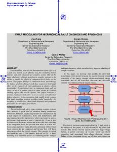
A finite language has application in fault diagnosis for sequential manufacturing systems, where a manufacturing process can be divided into a sequence of individual work cycles. During each cycle, a component finishes a finite number of operations, then resets to its initial value at the end of the cycle, and repeats the same operations in the next cycle. The transition behavior of each local component in one cycle can be modeled by a finite language. However, it is perhaps more interesting to know under what condition(s) CPLC terminates even though those languages may not be finite. Similar to the result in [9], [10], we can show that CPLC terminates in a tree-like network, and we can further provide the maximum number of rounds before termination. Proposition 9: If Gr is a tree then the termination condition holds no later than Round 2. A more general sufficient condition has been provided in [26], which says that if the network graph Gr contains a special spanning tree called a skeleton, which always exists and is unique if Gr is a tree, then CPLC terminates with arbitrary initial languages not necessarily regular. V. EXAMPLE—XEROX DC265ST PRINTER The following example illustrates distributed diagnosis with local consistency and global consistency. Fig. 7 is a schematic

depiction of a paper path model for the Xerox DC265ST printer consisting of 24 components, with permission of public release for academic use [31] from Xerox PARC. There are five sensors . Each sensor is used to record the leadinglabeled edge arrival time and the trailing-edge arrival time of each piece of paper. There are three motors in the system that transfer drive to rolls via gears, belts and clutches. Each box represents (normal and faulty) behavior of a local component in the paper path model. Arrows indicate interaction between components. The graph Gr of this distributed model is depicted in Fig. 8, where the label of each node is the component number corresponding to the component depicted in Fig. 7. The father–son relation is represented by the directed edges. We pick Feed Motor as the root node of Gr. The printing process can be divided into a sequence of work cycles, where a cycle starts when a piece of paper is fed into the system and ends when the paper is moved out. For simplicity we assume that at most one cycle is in progress at any time. Each local component is modeled as a finite language; the resetting operation is not explicitly modeled. It turns out that usually each local model has about 10–20 states, and some may have more (e.g., 50–60 states). If we use synchronous product to produce a centralized model, then the overall size would be enormous, and considering that there reaching a value between are 24 components each with size 10–20 states. The diagnosis

1932

IEEE TRANSACTIONS ON AUTOMATIC CONTROL, VOL. 50, NO. 12, DECEMBER 2005

TABLE IV

Given a set of local diagnoses on the supremal local (or global) support diagnosis is an element

based , a global such that

Fig. 8. Network graph of DC265ST printer model.

TABLE III

theory developed in this paper circumvents such a physically infeasible centralized model. Table III provides several possible observation scenarios in the paper path model for the Xerox DC265ST printer (Fig. 7) ,” and the corresponding local diagnoses, where “ “ ” and “ ” means component 14 is eito mean ther normal or wornout. We use that the leading edge Arrival time at Sensor 1 is normal, and to mean the trailing edge Arrival time at sensor 1 is normal. Other terms in the table can be interpreted accordingly. The CPU used in the following computation was a PIII 750 MHz and the computational time for the local diagnosis (its definition is given in Section III-B) in each row was s. Table III is to be interpreted as follows. After less than is obtained from sensor the first observation , local diagnosers report their local diagnoses as is obnormal. After the second observation tained, local diagnosers and report their local diagnoses as normal and so on. From Table III we can conclude that based are normal and on seven sensor readings, components are either normal or wornout. components

Notice that the set of all global diagnoses is isomorphic to a , which may be very large. For this reason, subset of in distributed diagnosis we do not compute global diagnoses. If the supremal global support is used then given a local diagnosis, each compound fault in that local diagnosis must be contained in at least one global diagnosis, but this may not be true if the supremal local support is used. In this sense, we say the supremal global support leads to a better diagnostic result than the supremal local support does. Although we do not recommend computing global diagnoses, in this example we compute them in order to make a quantitative comparison between diagnosis based on (regular) languages and diagnosis based on first-order logic. L2 is an executable kernel developed by NASA Ames Research Center [16]. The model-based diagnosis theory implemented by L2 has its origin in [6] and [24], and solves a diagnosis problem as a constraint satisfaction problem. The concept of global diagnosis in L2 is based on the concepts of conflict set and hitting set, but can be paraphrased in our terminologies: a global diagnosis is a set such that

The definition says that a global diagnosis in L2 is a collection of (compound) faults associated with a set of local components (not necessarily containing every local component) that can explain the observed symptom; the remaining local components are assumed to be normal. We can see that a indexed in is essenglobal diagnosis in L2 in its paraphrased version tially one global diagnosis in our definition. L2 seeks parsimoniously the subminimal global diagnoses, in the sense that should be as small as possible. In other words, if one global diis found, then every other global diagnosis, whose agnosis fault set contains all faults in will be discarded. In this sense, L2 has a smaller search space. Table IV shows the computational results for both methods.

SU AND WONHAM: GLOBAL AND LOCAL CONSISTENCIES IN DISTRIBUTED FAULT DIAGNOSIS

In Table IV, “ ” means the leading-edge arrival time at ” means the trailing-edge arrives late sensor is late, “ at sensor , “NPLD” stands for Number of Participating Local Diagnosers, “CT” is the Computational Time and “RL” means our regular-language-based approach. “NGD” is the Number of Global Diagnoses. In the column NGD the notation means that the RL method generates 21 global diagnoses and L2 generates 6 global diagnoses. We have checked that all fault candidates found by L2 are contained in the set of fault candidates generated by our method (as expected). Table IV indicates that as far as the global diagnosis is concerned, using regular languages to formulate and perform diagnosis can be much more efficient for this problem than L2. Such efficiency can be briefly explained as follows. In L2 the system model consists of a set of variables, each of which is associated with an appropriate domain, e.g., the velocity may take values from the set ; and a set of propositional logic expressions which describe the transition behavior of the system (i.e., the constraints imposed by the system’s behavior on those variables). During diagnosis an internal mechanism in L2 picks values for each variable and checks whether such value assignments satisfy the propositional logic constraints. If the assignment violates some constraint then a new assignment is picked. This process continues until either a user-defined number of (subminimal) fault candidates is reached or all (subminimal) fault candidates have been found, whichever occurs first. Significant time is spent on the process of picking an assignment and discarding a “bad” assignment. By contrast, in our language-based approach each local component is equivalent to a set of logic expressions in L2, and enumerates all possible assignments for that local component as strings. A computation based on natural projection and synchronous product submits a set of assignments for consistency checking, in place of the one-by-one assignment consistency checking in L2. That is why in Table IV the more sensors are involved, namely the more local components are involved in diagnosis, the greater the difference in computation time between L2 and our approach.

1933

framework enables us to capture features of distributed diagnosis which are invariant under choice of carrier. Second, we provide algorithms CPGC and CPLC to compute two types of supremal supports to facilitate distributed diagnosis. Although an idea similar to CPLC has appeared in the literature, e.g., [31] and [9], in this paper, we make a major improvement by introducing a binary relation (i.e., the father-son relation) to the set of local components, based on which we define the concept of round. In each round, pairwise communication is arranged in a particular order and direction, depending on whether the round number is even or odd. The advantage of such ordered communication is that we can tell how many rounds CPLC needs to run before its termination condition holds in situations when it is guaranteed to terminate. CPGC on the other hand is a new algorithm, which can achieve supremal global support in a finite number of synchronizations and projections. It turns out that CPLC may not always terminate. On the other hand, although CPGC may not be readily scalable, its termination is assured; furthermore to reduce time complexity of CPGC we can introduce hierarchical structure in the distributed diagnosis problem, where CPGC is applied at each level, as described in [29]. APPENDIX a) Proof of Proposition 1: Let . Since for each , clearly . Let . Then by definition of a global is globally consistent. Thus support set, we get that we have . Therefore , as claimed. b) Proof of Proposition 2: Suppose is . For each pair globally consistent. Let we have and . Then }, and the proposition follows. c) Proof of Proposition 3: Since is not empty, it has an index set . Suppose each element in takes the for some . Then, we form, perform the following construction:

VI. CONCLUSION In this paper we proposed two formulations to model consistency among local components in a distributed system, based on which we proposed two types of distributed diagnosis problems. We have achieved the following results. First, we provide a new general framework for distributed diagnosis. In this framework we model each local component as a language, and the interaction between each pair of components by strings from the set of their shared events. Such a framework is general enough to cover not only discrete-event systems, but also systems that can be modeled by propositional logic, e.g., [24], [6]. It is well known that each propositional logic expression can be converted into a BDD which can be treated as a finite-state automaton [15]. Compared with other frameworks for discrete-event systems, e.g., [10], [17], [2], and [9], ours is language-based and, thus, independent of the language carriers, e.g., automata or Petri nets. Although practical computation for a language has to be implemented on an appropriate language carrier, the language-based

Clearly, for each

, we have

So . By the construction of , for each we get . d) Proof of Proposition 4: As global consistency implies local consistency (by Proposition 2), we need only show the IF part. Suppose the graph Gr is a tree, and is locally consistent. We show that is globally consistent by induction on the size of . When is a singleton clearly the proposition is true. Suppose the proposition is true when has elements. Then we need to show that, no more than

1934

IEEE TRANSACTIONS ON AUTOMATIC CONTROL, VOL. 50, NO. 12, DECEMBER 2005

when has elements, it is also true. Since Gr is a tree and contains at least two nodes, let be a leaf node. such that Then there exists a unique node . Since the graph Gr is a tree with nodes, by the inductive hypothesis we have . Since is locally consistent, . Thus we have

father node of node . Since Gr is a tree, we have that is the only father node of . By CPLC we have

since is the unique father node of Let

. Then . Therefore,

For each we have

, owing to the local consistency property, On the other hand

Therefore, So the induction holds for , as required. e) Proof of Proposition 5: We use induction to show that (3) When and

, by the proposed procedure, . So . Suppose (3) is true when need to show that it also holds when dure

Therefore, (3) is true. Set computational procedure

. Then, we . By the proce-

. Then, by the proposed

and the proposition follows. f) Proof of Proposition 7: By [32, Lemma 2.2] we get that . Then by [32, Lemma 2.3] we have . Thus by definition of supremal local . support we have g) Proof of Proposition 9: To show that the termination condition holds at , it is sufficient to show that is locally consistent, namely for each . Clearly it is true for with . If then without losing generality, let node be the

, as required. REFERENCES

[1] A. Aghasaryan, E. Fabre, A. Benveniste, R. Boubour, and C. Jard, “A Petri net approach to fault detection and diagnosis in distributed systems,” in Proc. 1997 IEEE Conf. Decision and Control (CDC’97), Dec. 1997, pp. 720–725. [2] P. Baroni, G. Lamperti, P. Pogliano, and M. Zanella, “Diagnosis of large active systems,” Art. Intell., vol. 110, no. 1, pp. 135–183, May 1999. [3] J. Chen and R. J. Patton, Robust Model-Based Fault Diagnosis for Dynamic Systems. Boston, MA: Kluwer, 1999. [4] M. D. Cin, W. Hohl, and V. Sieh, “Hardware-supported fault tolerance for multiprocessors,” in Proc. Architektur von Rechensystemen ARCS’97. Rostock, Germany, 1997, pp. 13–22. [5] A. P. Dawid, “Applications of a general propagation algorithm for probabilistic expert systems,” Statist. Comput., vol. 2, pp. 25–36, 1992. [6] J. de Kleer and B. C. Williams, “Diagnosing multiple faults,” Art. Intell., vol. 32, pp. 97–130, 1987. [7] R. Debouk, S. Lafortune, and D. Teneketzis, “Coordinated decentralized protocols for failure diagnosis of discrete event systems,” Discrete Event Dyna. Syst.: Theory Appl., vol. 10, no. 1/2, pp. 33–86, Jan. 2000. [8] R. Diestel, Graph Theory, 2nd ed. New York: Springer-Verlag, 2000. [9] E. Fabre, A. Benveniste, S. Haar, and C. Jard, “Distributed monitoring of concurrent and asynchronous systems,” J. Discrete Event Dyna. Syst., vol. 15, no. 1, pp. 33–84, Mar. 2005. [10] E. Fabre, A. Benveniste, and C. Jard, “Distributed diagnosis for large discrete event dynamic systems,” in Proc. 15th IFAC World Congr., Barcelona, Spain, Jul. 2002. [11] E. Fabre, A. Benveniste, C. Jard, L. Ricker, and M. Smith, “Distributed state reconstruction for discrete event systems,” in Proc. 39th IEEE Conf. Decision and Control (CDC’00), Sydney, NSW, Australia, Dec. 2000, pp. 2252–2257. [12] R. G. Gallager, Low-Density Parity Check Codes. Cambridge, MA: MIT Press, 1963. [13] C. N. Hadjicostis and G. C. Verghese, “Monitoring discrete event systems using Petri net embeddings,” in Springer-Verlag Lecture Notes in Computer Science. New York: Springer-Verlag, Jun. 1999, vol. 1639, pp. 188–207. [14] J. E. Hopcroft and J. D. Ullman, Introduction to Automata Theory, Languages and Computation. Reading, MA: Addison-Wesley, 1979. [15] N. Klarlund, “Mona & Fido: The logic-automaton connection in practice,” in Springer-Verlag Lecture Notes in Computer Science. New York: Springer-Verlag, 1997, vol. 1414, pp. 311–326. [16] J. Kurien and P. P. Nayak, “Back to the future with consistency based trajectory tracking,” in Proc. 17th National Conf. Artificial Intelligence (AAAI 2000), Austin, TX, Jul. 2000, pp. 370–377. [17] G. Lamperti, M. Zanella, and P. Pogliano, “Diagnosis of active systems by automata-based reasoning techniques,” Appl. Intell., vol. 12, no. 3, pp. 217–237, May 2000. [18] N. A. Lynch, Distributed Algorithms. San Francisco, CA: Morgan Kaufmann, 1996.

SU AND WONHAM: GLOBAL AND LOCAL CONSISTENCIES IN DISTRIBUTED FAULT DIAGNOSIS

[19] R. McEliece, D. MacKey, and J. Cheng, “Turbo decoding as an instance of Pearl’s ‘belief propagation’ algorithm,” IEEE J. Select. Areas Commun., vol. 16, no. 2, pp. 140–152, Feb. 1998. [20] R. Mohr and T. Henderson, “Arc and path consistency revisited,” Art. Intell., vol. 28, pp. 225–233, 1986. [21] J. Pearl, Probabilistic Reasoning in Intelligent Systems: Networks of Plausible Inference. San Mateo, CA: Morgan Kaufmann, 1988. [22] Y. Pencolé and M.-O. Cordier, “A formal framework for the decentralised diagnosis of large scale discrete event systems and its application to telecommunication networks,” Art. Intell., vol. 164, no. 1–2, pp. 121–170, May 2005. [23] Y. Peng and J. A. Reggia, Abductive Inference Models for Diagnostic Problem Solving. New York: Springer-Verlag, 1990. [24] R. Reiter, “A theory of diagnosis from first principles,” Art. Intell., vol. 32, pp. 57–95, 1987. [25] M. Sampath, R. Sengupta, S. Lafortune, K. Sinnamohideen, and D. Teneketzis, “Failure diagnosis using discrete-event models,” IEEE Trans. Control Syst. Technol., vol. 4, no. 2, pp. 105–124, Feb. 1996. [26] J. G. Thistle and R. Su, “Uncomputability of supremal local supports and effective consistent distributed diagnosis,” Dept. Elect. Comput. Eng., Univ. Waterloo, Waterloo, ON, Canada, Tech. Rep. 2005–06, Apr. 2005. [27] R. Su and W. M. Wonham, “Decentralized fault diagnosis for discrete-event systems,” in Proc. 2000 CISS, Princeton, NJ, Mar. 2000, pp. TP1-1–TP1-6. , “An algorithm to achieve local consistency in distributed di[28] agnosis,” in Proc. 43th IEEE Conf. Decision and Control (CDC’04), Nassau, Bahamas, Dec. 2004, pp. 998–1003. , “Hierarchical distributed diagnosis under global consistency,” in [29] Proc. 2004 IFAC Workshop on Discrete Event Systems (WODES’04), Reims, France, Sep. 2004, pp. 157–162. [30] , “Undecidability of termination of CPLC for computing supremal local support,” in Proc. 42nd Annu. Allerton Conf. Communication, Control, and Computing, Monticello, IL, Sep. 2004. [31] R. Su, W. M. Wonham, J. Kurien, and X. Koutsoukos, “Distributed diagnosis for qualitative systems,” in Proc. 6th Int. Workshop on Discrete Event Systems (WODES’02), Zaragoza, Spain, Oct. 2002, pp. 169–174. [32] R. Su, “Distributed diagnosis for discrete-event systems,” Ph.D. dissertation, ECE Dept., Univ. Toronto, Toronto, ON, Canada, 2004. [33] J. G. Thistle and R. Su, “Uncomputability of supremal local supports in distributed diagnosis,” in Proc. Joint 44th IEEE Conf. Decision and Control (CDC) and European Control Conference (ECC), Seville, Spain, Dec. 2005. [34] M. J. Wainwright, T. Jaakkola, and A. S. Willsky, Tree Consistency and Bounds on the Performance of the Max-Product Algorithm and its Generalizations. Cambridge, MA: Laboratory for Information and Decision Systems, 2002. [35] R. Weigel and B. Faltings, “Compiling constraint satisfaction problems,” Art. Intell., vol. 115, no. 2, pp. 257–287, 1999. [36] K. C. Wong and W. M. Wonham, “On the computation of observers in discrete-event systems,” Discrete Event Dyna. Syst.: Theory Appl., vol. 14, no. 1, pp. 55–107, Jan. 2004. [37] W. M. Wonham. (2004) Supervisory Control of Discrete-Event Systems [Online]. Available: www.control.utoronto.ca/DES

1935

[38]

, (2004) Design Software [Online]. Available: www.control. utoronto.ca/DES [39] M. Yokoo, E. H. Durfee, T. Ishida, and K. Kuwabara, “The distributed constraint satisfaction problem: Formalization and algorithms,” IEEE Trans. Knowledge Data Eng., vol. 10, no. 5, pp. 673–685, Oct. 1998. [40] S. H. Zad, R. H. Kwong, and W. M. Wonham, “Fault diagnosis in discrete-event systems: Framework and model reduction,” IEEE Trans. Autom. Control, vol. 48, no. 7, pp. 1199–1212, Jul. 2003.

R. Su received the B.Eng. degree in automatic control from University of Science and Technology of China, in 1997, and the M.A.Sc. and Ph.D. degrees in electrical and computer engineering from University of Toronto, Toronto, ON, Canada, in 2000 and 2004, respectively. From 2004 to 2005, he was associated with the Electrical and Computer Engineering Department, University of Waterloo, Waterloo, ON, Canada. Currently, he is a Postdoctoral Fellow in the Mathematics and Computer Science Department, Eindhoven University of Technology, The Netherlands. His current research interests include fault diagnosis and supervisory control of discrete-event systems, computability and complexity analysis, and optimization theories.

W. M. Wonham (M’64–SM’76–F’77–LF’00) received the B.Eng. degree in engineering physics from McGill University, Montreal, QC, Canada, in 1956, and the Ph.D. degree in control engineering from the University of Cambridge, Cambridge, U.K., in 1961. From 1961 to 1969, he was associated with several U.S. research groups in control. Since 1970, he has been a Faculty Member in Systems Control, with the Department of Electrical and Computer Engineering, the University of Toronto, Toronto, ON, Canada. His research interests have included stochastic control and filtering, geometric multivariable control, and discrete-event systems. He is the author of Linear Multivariable Control: A Geometric Approach (Springer-Verlag, 1985) and coauthor (with C. Ma) of Hierarchical Control of State Tree Structures (Springer-Verlag, 2005). Dr. Wonham is a Fellow of the Royal Society of Canada, and a Foreign Associate of the (U.S.) National Academy of Engineering. In 1987 he received the IEEE Control Systems Science and Engineering Award and in 1990 was Brouwer Medallist of the Netherlands Mathematical Society. In 1996, he was appointed University Professor in the University of Toronto, and in 2000, University Professor Emeritus.