BIOC-06881; No of Pages 8 Biological Conservation xxx (2016) xxx–xxx
Contents lists available at ScienceDirect
Biological Conservation journal homepage: www.elsevier.com/locate/bioc
Short Communication
Global biodiversity monitoring: From data sources to Essential Biodiversity Variables Vânia Proença a,⁎, Laura Jane Martin b, Henrique Miguel Pereira c,d,e, Miguel Fernandez c,f, Louise McRae g, Jayne Belnap h, Monika Böhm g, Neil Brummitt i, Jaime García-Moreno j, Richard D. Gregory k, João Pradinho Honrado e,l, Norbert Jürgens m, Michael Opige n, Dirk S. Schmeller o,p, Patrícia Tiago e,q, Chris A.M. van Swaay r a
MARETEC, Instituto Superior Técnico, Universidade de Lisboa, Av. Rovisco Pais 1, 1049-001 Lisboa, Portugal Harvard University, Center for the Environment, Harvard University, Cambridge, MA 02138, USA c German Centre for Integrative Biodiversity Research (iDiv) Halle-Jena-Leipzig, Deutscher Platz 5e, 04103 Leipzig, Germany d Institute of Biology, Martin Luther University Halle-Wittenberg, Am Kirchtor 1, 06108 Halle (Saale), Germany e CIBIO/InBIO - Rede de Investigação em Biodiversidade e Biologia Evolutiva, Universidade do Porto, Campus Agrário de Vairão, 4485-601 Vairão, Portugal f Instituto de Ecología, Universidad Mayor de San Andrés, Campus Universitario, Cota-cota, Calle 27, La Paz, Bolivia g Institute of Zoology, Zoological Society of London, Regent's Park, London NW1 4RY, UK h U. S. Geological Survey, Southwest Biological Science Center, Moab, UT 84532, USA i Department of Life Sciences, Natural History Museum, Cromwell Road, London SW7 5BD, UK j ESiLi Consulting. Het Haam 16, 6846 KW, Arnhem, The Netherlands k RSPB Centre for Conservation Science, RSPB, The Lodge, Sandy, Bedfordshire, SG19 2DL, UK l Faculdade de Ciências, Universidade do Porto, Rua do Campo Alegre, FCUP-Edificio FC4 (Biologia), 4169-007 Porto, Portugal m Biodiversity, Evolution and Ecology (BEE), Biocenter Klein Flottbek, University of Hamburg, Ohnhorststrasse 18, 22609 Hamburg, Germany n Nature Uganda, The East Africa Natural History Society, P. O. Box 27034, Katalima Crescent, Naguru, Kampala, Uganda o Helmholtz Center for Environmental Research, UFZ, Department of Conservation Biology, Permoserstrasse 15, 04318 Leipzig, Germany p ECOLAB, Université de Toulouse, UPS, INPT, Toulouse, France q Centre for Ecology, Evolution and Environmental Changes (CE3C), Faculdade de Ciências, Universidade de Lisboa, 1749-016 Lisbon, Portugal r Dutch Butterfly Conservation, P.O. Box 506, 6700 AM Wageningen, Netherlands b
a r t i c l e
i n f o
Article history: Received 26 February 2016 Received in revised form 15 June 2016 Accepted 11 July 2016 Available online xxxx Keywords: Primary biodiversity observations Biodiversity monitoring schemes Essential Biodiversity Variables GEO BON Global biodiversity monitoring Living Planet Index
a b s t r a c t Essential Biodiversity Variables (EBVs) consolidate information from varied biodiversity observation sources. Here we demonstrate the links between data sources, EBVs and indicators and discuss how different sources of biodiversity observations can be harnessed to inform EBVs. We classify sources of primary observations into four types: extensive and intensive monitoring schemes, ecological field studies and satellite remote sensing. We characterize their geographic, taxonomic and temporal coverage. Ecological field studies and intensive monitoring schemes inform a wide range of EBVs, but the former tend to deliver short-term data, while the geographic coverage of the latter is limited. In contrast, extensive monitoring schemes mostly inform the population abundance EBV, but deliver long-term data across an extensive network of sites. Satellite remote sensing is particularly suited to providing information on ecosystem function and structure EBVs. Biases behind data sources may affect the representativeness of global biodiversity datasets. To improve them, researchers must assess data sources and then develop strategies to compensate for identified gaps. We draw on the population abundance dataset informing the Living Planet Index (LPI) to illustrate the effects of data sources on EBV representativeness. We find that long-term monitoring schemes informing the LPI are still scarce outside of Europe and North America and that ecological field studies play a key role in covering that gap. Achieving representative EBV datasets will depend both on the ability to integrate available data, through data harmonization and modeling efforts, and on the establishment of new monitoring programs to address critical data gaps. © 2016 Published by Elsevier Ltd.
⁎ Corresponding author. E-mail addresses:
[email protected] (V. Proença),
[email protected] (L.J. Martin),
[email protected] (H.M. Pereira),
[email protected] (M. Fernandez),
[email protected] (L. McRae),
[email protected] (J. Belnap),
[email protected] (M. Böhm),
[email protected] (N. Brummitt),
[email protected] (J. García-Moreno),
[email protected] (R.D. Gregory),
[email protected] (J.P. Honrado),
[email protected] (N. Jürgens),
[email protected] (M. Opige),
[email protected] (D.S. Schmeller),
[email protected] (P. Tiago),
[email protected] (C.A.M. van Swaay).
http://dx.doi.org/10.1016/j.biocon.2016.07.014 0006-3207/© 2016 Published by Elsevier Ltd.
Please cite this article as: Proença, V., et al., Global biodiversity monitoring: From data sources to Essential Biodiversity Variables, Biological Conservation (2016), http://dx.doi.org/10.1016/j.biocon.2016.07.014
2
V. Proença et al. / Biological Conservation xxx (2016) xxx–xxx
1. Introduction In 2010, the parties of the United Nations Convention on Biological Diversity (CBD) adopted the Aichi Targets for 2020, which include goals such as “reducing the direct pressures on biodiversity” and “improving the status of biodiversity by safeguarding ecosystems, species and genetic diversity.” A mid-term assessment of the Aichi Targets (Tittensor et al. 2014) suggested that while actions to counteract the decline of biodiversity have increased, so too have pressures, and there has been a further deterioration in the state and trends of biodiversity. In order to be effective, actions towards the Aichi targets will have to be supported by updated information on regional and global patterns of biodiversity change, on drivers of biodiversity change, and on the effectiveness of conservation policies (Pereira and Cooper, 2006; Scholes et al., 2012; Tittensor et al., 2014). However, such data are either missing or not readily accessible, as reflected by the lack of quantitative data on biodiversity change in two-thirds of the 4th national reports submitted by Parties to the CBD (Bubb et al., 2011), and this affects the indicators too (Tittensor et al., 2014). Researchers and conservation managers hoping to assess biodiversity change at the regional or global level face a number of obstacles. First, the geographic coverage of extant biodiversity monitoring programs is insufficient and uneven (Pereira et al., 2010, 2012). In particular, biodiversity monitoring efforts and ecological fieldwork are biased towards developed countries in temperate regions (McGeoch, et al. 2010; Martin et al., 2012; Hudson et al., 2014). Second, monitoring schemes are typically not implemented at regional scales and few deliver long-term data, making it difficult to monitor biodiversity change across space and time (Schmeller, 2008; Hudson et al. 2014; McGeoch et al., 2015; but see Jürgens et al., 2012). In an effort to optimize biodiversity monitoring initiatives, the Group on Earth Observations Biodiversity Observation Network (GEO BON; Scholes et al., 2012) has developed the concept of Essential Biodiversity Variables (EBVs) that could form the basis of efficient and coordinated monitoring programs worldwide (Pereira et al., 2013). The EBV concept was inspired by the Essential Climate Variables that guide
implementation of the Global Climate Observing System by Parties to the UN Framework Convention on Climate Change. EBVs are state variables that stand between primary observations (i.e., raw data) and high level indicators (e.g., the Living Planet Index (Collen et al., 2009)), and may represent essential aspects of biodiversity (from genetic composition to ecosystem functioning) or may be integrated with other EBVs or with other types of data, such as data on drivers and pressures, to deliver high-level indicators (Pereira et al., 2013; GEO BON 2015a). The aim of the EBV framework is to identify a minimum set of variables that can be used to inform scientists, managers and the public on global biodiversity change. In a first attempt to identify a minimum set of EBVs, GEO BON aggregated candidate variables into six classes: “genetic composition,” “species populations,” “species traits,” “community composition,” “ecosystem structure,” and “ecosystem function” (Pereira et al., 2013). Recently, Geijzendorffer et al. (2015) compared the EBV framework with indicators currently used for reporting biodiversity information by seven biodiversity policy instruments. They found that the current suite of biodiversity indicators does not incorporate EBV classes equally. For instance, some EBV classes, like “species populations,” were well represented in current indicators, while others, like “genetic composition,” were not. This asymmetry in EBV coverage is related to biases in indicator selection, and ultimately to biases in extant biodiversity monitoring data, as indicator selection is often driven by data availability for reasons of feasibility (Geijzendorffer et al., 2015). Hence, the current set of indicators misses important biodiversity facets, due to gaps in primary data. Instead, monitoring efforts should be driven by the information needs of selected indicators. The EBV framework could become an important tool towards that end, by promoting costefficient approaches (Pereira et al. 2013, Fig.1). This article aims to discuss how primary data sources affect the representativeness of current EBV datasets. That is, if available, are primary data well distributed across spatial and temporal scales of interest to provide meaningful measures on biodiversity change? Do data cover a diverse range of species groups? Previous studies have identified the existence of geographic and taxonomic biases in data
Fig. 1. Data flow from different data sources of primary biodiversity observations into EBVs, followed by EBVs input to build biodiversity indicators used to monitor Aichi targets. The width of the arrows represents the relative input of each source into EBVs and of EBVs into indicators. Only a few EBVs are shown to illustrate the flow of data from sources to biodiversity indicators, the relative contribution of each source to inform indicators will vary depending on the chosen indicators. LPI – Living Planet Index, RLI – Red List Index.
Please cite this article as: Proença, V., et al., Global biodiversity monitoring: From data sources to Essential Biodiversity Variables, Biological Conservation (2016), http://dx.doi.org/10.1016/j.biocon.2016.07.014
V. Proença et al. / Biological Conservation xxx (2016) xxx–xxx
availability (e.g., Boakes et al., 2010, Pereira et al., 2010; Martin et al., 2012; Hudson et al., 2014; Velasco et al., 2015). Data asymmetries will be a barrier to effective policy responses (Pereira et al., 2010; Geijzendorffer et al., 2015). Hence, a first step towards improving global EBV datasets is to assess the underlying data sources and to identify existing biases. Only then will it be possible to develop strategies to cover data gaps and to optimize the use of available data. Here we demonstrate the links between data sources, EBVs and indicators. We classify the main sources of primary observations of terrestrial biodiversity as: (1) extensive monitoring schemes, (2) intensive monitoring schemes, (3) ecological field studies, and (4) satellite remote sensing. We define each class and its scope by its geographic, taxonomic, and temporal coverage. We then analyze the dataset informing the Living Planet Index indicator (LPI; Collen et al., 2009) to illustrate the effects of primary data sources on EBV representativeness. The LPI is one of the most complete datasets of biodiversity observations on population abundances. Therefore, the identified gaps should provide an overview of the challenges in building a spatially explicit and globally representative dataset for the population abundance EBV. Finally, we discuss how biases in data sources affect the representativeness of biodiversity monitoring datasets and we suggest methods to address data gaps. 2. Types of primary data sources Sources of primary biodiversity observations can be characterized by their geographic, taxonomic, and temporal coverage (Couvet et al., 2011). In order to develop a typology we consider the following features: (1) the coverage density (geographic coverage); (2) the observation effort per site and the sampling frequency (impacting on taxonomic coverage, seasonal and day/night biases); and (3) the length of time series (temporal coverage). Along these dimensions source types fall into four categories: extensive monitoring schemes, intensive monitoring schemes, ecological field studies and remote sensing (Table 1). Extensive monitoring schemes maximize geographic coverage at the expense of sampling effort per site, expressed as the number of ecosystem variables or functional groups monitored and/or sampling frequency (Couvet et al., 2011). A widespread spatial coverage is often achieved through the simplification of the observation effort per site, namely by focusing on a target species group. This trade-off not only reduces the costs per site but also enables volunteer engagement (Couvet et al., 2011; Schmeller et al., 2009). Consequently, extensive monitoring schemes tend to focus on popular and conspicuous species groups, such as birds and butterflies. Intensive monitoring schemes, meanwhile, invest in the effort per site at the expense of geographic coverage. The goal of intensive schemes is to capture ecological responses to environmental change, by monitoring ecosystem functioning and species interactions (Couvet et al., 2011; Jürgens et al., 2012). Overall, extensive monitoring schemes are best suited for monitoring trends in species distribution and abundance whereas intensive schemes can generate data for multiple EBVs. On the other hand, the larger and denser the network of sites in an extensive monitoring scheme, the better the data scalability (i.e., the ability to aggregate data at multiple scales). Both extensive and intensive
3
monitoring schemes provide long-term data series and both can spread over a large spatial extent, but with different levels of coverage density. Moreover, although the above categorization is useful for data comparison purposes, it is important to note that because the geographic coverage of monitoring schemes falls along a continuous gradient, the threshold between extensive and intensive monitoring schemes is not always precise. For instance, while intensive schemes are applied in LTER sites, the ILTER network, which aggregates national LTER networks (i.e., a network of networks), has a widespread global coverage composed by a vast number of sites (Vanderbilt, et al. 2015; Table 2). In recent years, data from ecological field studies and satellite remote sensing have been used increasingly as aggregated datasets have become more accessible (Karl et al., 2013; Hudson et al., 2014; Pimm et al., 2014). Ecological field studies, here defined as experimental or observational studies located outdoors (Martin et al., 2012), are numerous but often conducted independently of each other. Despite the large spatial coverage achieved when independent studies are aggregated (e.g., Hudson et al., 2014), data scalability is constrained by the fact that ecological field studies do not share a common design or data recording scheme. Also, compared with the other sources of biodiversity data, ecological field studies tend to deliver short-term data series (Hudson et al., 2014). Yet, because ecological field studies explore different research questions and report many different types of data, they also cover multiple EBV classes. Similarly, citizen science generates numerous opportunistic data on species observations. Despite their large number and spatial coverage, the use of these data has been limited by quality issues, namely the lack of sampling protocols. Recent developments in data correction methods promise to allow researchers to use opportunistic citizen science data to monitor species distribution trends (van Strien et al., 2013; Isaac et al., 2014). Satellite remote sensing can deliver long-term data series with a high sampling frequency and extensive geographic coverage. Satellite remote sensing can be distinguished from other types of remote sensing, such as aircraft or drones, by its global and continuous coverage. Moreover, and for sake of simplicity, the latter can be framed within the techniques used in long-term monitoring schemes and ecological field studies. Although satellite remote sensing data are often vegetation-related, and are typically used to monitor ecosystem function and ecosystem structure EBVs (e.g., NPP, ecosystem extent and fragmentation), there is some potential to monitor a broader range of EBVs (Turner, 2014; Skidmore et al., 2015; O'Connor et al., 2015; Pettorelli et al., 2016). Still, the ongoing development of techniques for remote sensing data collection and processing creates challenges for the aggregation of time series, but also opportunities for the use of these data in biodiversity monitoring (Pasher et al., 2013; Skidmore et al., 2015). Moreover, while the resolution of satellite imagery is rapidly improving, enabling a more diverse range of applications, the high costs and time needed for data processing could be a constraint (Pasher et al., 2013). This is reflected in the paucity of map products, despite frequent data collection, and stresses the need for international and multidisciplinary approaches that harness the use of earth observation data (Pasher et al., 2013). In addition, the production of EBV datasets from satellite data will require coordinated action from data providers, biodiversity and remote sensing experts, and policy makers (Pettorelli et al., 2016).
Table 1 Qualitative assessment of the key attributes of primary sources of global biodiversity monitoring data and their coverage of EBV classes.
Spatial coverage density Effort per site Time series Sampling frequency Main biases or limitations EBV classes
Extensive schemes
Intensive schemes
Ecological field studies
Remote sensing
High Low Long-term Moderate Often directed to common, conspicuous or charismatic taxa Species populations, Community composition
Low High Long-term High Low density of network sites (i.e. few sites) Multiple EBVs
High Low to high Short-term Moderate to high Short-term data series; diverse field protocols Multiple EBVs
Very high Low Medium to long-term Very high Low resolution data; often vegetation-related variables measured at the ecosystem level Ecosystem structure, Ecosystem function
Please cite this article as: Proença, V., et al., Global biodiversity monitoring: From data sources to Essential Biodiversity Variables, Biological Conservation (2016), http://dx.doi.org/10.1016/j.biocon.2016.07.014
4
V. Proença et al. / Biological Conservation xxx (2016) xxx–xxx
Biodiversity monitoring datasets may combine primary biodiversity observations from a single source, from different sources of the same type, or from different sources of different types (Fig. 1). The global map of 21st century forest cover change by Hansen et al. (2013) is an example of the first case. It combines time series of Landsat data to monitor forest cover change at the global scale. An example of the second case is the global Wild Bird Index (WBI; Gregory et al., 2005; Gregory & van Strien 2010) dataset, which currently combines the species abundance data delivered by the Pan-European Common Bird Monitoring Scheme and the North American Breeding Bird Survey (Table 2). The Living Planet Index (LPI; Collen et al., 2009) dataset provides an example of the last case, as it combines data from extensive schemes, intensive schemes, and ecological field studies (see next section). Moreover, primary biodiversity observations may be compiled and made available through secondary sources, such as databases (e.g., the PREDICTS database (Hudson et al., 2014)), data repositories, or institutional reports. 3. The data sources behind the Living Planet Index The LPI is among the best established indicators of the state of global biodiversity (Butchart et al., 2010; Tittensor et al., 2014). It monitors changes in population abundance relative to a 1970 baseline using time series of vertebrate populations across the globe (Collen et al., 2009; Fig. 2a). The underlying dataset aggregates time series for N16,000 populations of over 3600 species of vertebrates (http://www. livingplanetindex.org/, accessed 14.06.2016) and is one of the most complete datasets on the population abundance EBV (Collen et al., 2009; Tittensor et al., 2014). New data are added to the dataset as they become available. A candidate population is included in the dataset only if data on population size are available for at least two years and data were always collected using the same method on the same population throughout the time series (Collen et al., 2009). Data generated by different types of primary sources, namely, extensive schemes, intensive schemes, and ecological field studies, are collected from a variety of available sources, including published scientific literature, on-line databases and gray literature (Collen et al., 2009). Therefore, the LPI dataset emerges from ongoing data survey and collection. Here we analyze two subsets of the LPI dataset, the subset of terrestrial birds (4406 time series of 1025 species, time interval: 1900–2013) and the subset of terrestrial mammals (2229 time series of 438 species, time interval: 1900–2014). We use information on the length of the time series (i.e., the time interval between the start and end year), number of data points (i.e., number of measurements made during the time interval) and the purpose of primary data collection
(i.e., baseline monitoring, conservation or natural resource management, or population studies) to infer if data originate from long-term monitoring schemes (i.e., extensive and intensive schemes) or from ecological field studies. Lindenmayer and Likens (2010) proposed a minimum time series length of 10 years to qualify a study as long-term, while emphasizing that this is an operational criterion and that the adequate threshold depends on the taxa or ecosystem processes being monitored. For the purpose of our analysis, we assigned long-term monitoring schemes to long-term time series, here defined by a minimum of 10 data points if the series started after 1995, or a minimum of 15 data points if the series started in 1995 or before. We do not discriminate extensive from intensive schemes because the dataset does not provide precise information on the number of sampling sites and spatial coverage of the primary source. For that reason, we do not discuss the relative contribution of these source types to the LPI. Ecological field studies were assigned to short-term time series of non-baseline monitoring studies. Moreover, recently started time series collected for baseline monitoring purposes could evolve in the future into long-term time series. Results show that for both birds and mammals a large share of the available data stems from temperate regions, in particular Europe and North America (Fig. 2b-c); in the case of mammals, the equatorial region is also better represented than other world regions. In order to correct for geographic biases, a method of proportional weighting is currently applied to the data when calculating the global LPI (McLellan et al., 2014). Regarding the temporal coverage, long-term time series comprise a large share of bird population data but are largely confined to temperate regions (Figs. 2b, 3a, Appendix A). On the other hand, short-term time series dominate for mammals across all world regions (Figs. 2c, 3b, Appendix A). Relatedly, both species groups are weakly represented by long-term data in tropical regions. Finally, the breadth of the taxonomic coverage also differs between the two species groups. Most sources of bird time-series target multiple taxonomic orders, while in the case of mammals, with the exception of the equatorial region, most sources target a single order (Figs. 2b-c, 3), and of these 60% target a single species (Appendix B). The bias towards the northern hemisphere is particularly accentuated in the case of birds, where extensive monitoring schemes, such as the North American Breeding Bird Survey and the Pan-European Common Bird Monitoring Scheme (Table 2), deliver many of the long-term (multi order) data on bird populations (Fig. 3a, Appendix C). Efforts are being pursued to implement similar schemes in gap regions, particularly in African countries (BirdLife International, 2013). Once implemented, these schemes will contribute to reducing the data gap and consequently the geographic bias. Notwithstanding, the International Waterbird Census (Table 2) has global coverage, operating in 143 countries and building
Table 2 Examples of large scale (i.e., international or continental) extensive (E) and intensive (I) monitoring schemes. Monitoring schemea
Type
Coverage
Network
Species groups
Start year
Sampling frequency
Pan-European Common Bird Monitoring Scheme (PECBMS) Breeding Bird Survey (BBS) International Waterbird Census (IWC) Great Backyard Bird Count (GBBC) National Butterfly Monitoring Schemes (BMS) Important Bird and Biodiversity Areas (IBAs) International Long-Term Ecological Research Network (ILTER) National Ecological Observation Network (NEON) Biodiversity Monitoring Transect Analysis in Africa (BIOTA) Tropical Ecology Assessment & Monitoring network (TEAM)
E E E E E E I I I I
Europe North America Global Global Europe Global Global U.S. Africa Africa, Asia, Latin America
N12,000 sites N1000 sites N25,000 sites N137,000 checklistsb 2000 sites N3000 sites N600 sites e 60 terrestrial sites 4 regional transects 16 sites
Birds Birds Birds Birds Butterflies Birds Unrestricted Unrestricted Unrestricted Plants, Mammals, Birds
1980 1966 1967 2013c 1990 1994 d 1993 2011 1999 2009
Annual Annual Annual Annual Annual Annual Depends on species group Depends on species group Depends on species group Annual (dry season)
a Websites: PECBMS (http://www.ebcc.info/); BBS (https://www.pwrc.usgs.gov/bbs/); IWC (http://www.wetlands.org/); GBBC (http://gbbc.birdcount.org/); BMS (http:// www.bc-europe.eu/); IBA (http://www.birdlife.org/); NEON (http://www.neoninc.org/); ILTER (http://www.ilternet.edu/); BIOTA (http://www.biota-africa.org/); TEAM (http://www.teamnetwork.org). b GBBC is a citizen science project, participants reported 137,998 checklists in 2013. c Global scope since 2013, running in US since 1998. d Some national LTER networks started before ILTER (e.g., US LTER started in 1980). e NEON operates 20 core terrestrial sites +40 relocatable terrestrial sites.
Please cite this article as: Proença, V., et al., Global biodiversity monitoring: From data sources to Essential Biodiversity Variables, Biological Conservation (2016), http://dx.doi.org/10.1016/j.biocon.2016.07.014
V. Proença et al. / Biological Conservation xxx (2016) xxx–xxx
5
Fig. 2. Global distribution of terrestrial Living Planet Index (LPI) time series over a map of forest change (a), the size of each dot is proportional to the number of populations monitored (adapted from Pereira et al. 2010 and Hansen et al. 2013). Forest change is shown 1 km-pixels and includes areas of forest loss, forest gain and areas of both loss and gain; Latitudinal distribution of LPI time series of population abundance of terrestrial birds (b) and mammals (c) classified by time series length and taxonomic coverage of the data source: STSO short-term single order, STMO - short-term multiple order, LTSO - long-term single order, LTMO - long-term multiple order (see Section 3 for a definition of each class). The midpoints of the latitude classes are shown. Source: ZSL/WWF, Hansen et al. 2013.
on the contribution of thousands of volunteers (Wetlands International, 2016). Long-term time series on mammal population abundances also show a bias towards the northern hemisphere, with data, equally distributed across North America, Europe and Asia. For this species group, ecological field studies seem to be providing more long-term data than monitoring schemes (Fig. 3b, Appendix C). Concurrently, short-term ecological field studies constitute an alternative, relatively abundant and globally distributed source of time series of population abundance. Ecological field studies deliver a great part of the available time series of mammal population abundance and are essential to complement bird monitoring data (Fig. 3, Appendix C). However, differences in sampling protocols affect data scalability across space and time, hence limiting the full use of primary data (Henry et al., 2008). Furthermore, while the aggregation of data from different sources confers a broad taxonomic coverage (within the vertebrates) to the LPI dataset, many of the sources, particularly for mammals, target a single species or order (Figs. 2c, 3b, Appendix B). This represents a limitation if community-level responses are relevant for monitoring the impacts of environmental change, such as the assessment of trophic chain effects or the identification of potential “loser” and “winner” species. Finally, the global distribution of post-2010 data (Appendix D) suggests that the commitment to the Aichi Targets has yet to be followed by the implementation of new monitoring programs in gap regions.
4. Improving the representativeness of EBV datasets The goal of global biodiversity monitoring is to measure biodiversity responses to environmental change. This goal implies the use of time series, in particular long-term data capable of capturing on-going changes through time (Scholes et al., 2012; Han et al., 2014). Data must also be scalable, so that biodiversity change can be assessed across scales and compared between sites (Pereira and Cooper, 2006; Han et al., 2014; Latombe et al., this issue), and taxonomically representative, so that a more complete understanding of biodiversity change, which includes community level changes, can be achieved. Here, we have examined what is arguably the most representative global dataset of population abundance, a dataset produced to inform the LPI indicator. The analysis revealed two types of data biases, geographic (i.e., more data from temperate regions) and temporal (i.e., a predominance of short-term time series). Moreover, the taxonomic coverage is currently restricted to vertebrates, which, despite being the best known taxonomic group, represent only a small fraction of life on earth (Pereira et al., 2012). Long-term monitoring schemes for non-vertebrate taxa are still scarce and should be targeted by future monitoring efforts. New programs, such as the National Butterfly Monitoring Schemes in Europe (Table 2), are already helping to address this gap. The selection of target taxa is challenging however. First, it is not feasible to select a comprehensive set of taxa for global
Please cite this article as: Proença, V., et al., Global biodiversity monitoring: From data sources to Essential Biodiversity Variables, Biological Conservation (2016), http://dx.doi.org/10.1016/j.biocon.2016.07.014
6
V. Proença et al. / Biological Conservation xxx (2016) xxx–xxx
Fig. 3. Reasons for primary data collection of LPI time series of birds (a) and mammals (b). Time series are classified by their length and the taxonomic coverage of the data source. Conserv/NRM studies include studies on conservation and natural resource management; population studies include studies on population dynamics and studies tracking declining species. STSO - short-term single order, STMO - short-term multiple order, LTSO - long-term single order, LTMO - long-term multiple order (see Section 3 for a definition of each class). Source: ZSL/WWF.
monitoring purposes, and second, taxon groups respond differently to pressures and differ in their distribution patterns. Therefore, taxon selection should follow pragmatic criteria, such as the feasibility of monitoring at the global scale and their functional role in ecosystem processes (GEO BON, 2010). Generating new data through the establishment of new monitoring schemes is one of two main approaches to enhance the representativeness of EBV datasets. The second approach is through data integration, that is, by making the best use of data generated by ecological field studies and monitoring schemes, from local to regional scales, and by satellite remote sensing. The establishment of new monitoring programs will be particularly important in the case of gap regions and taxa for which data is scarce or virtually missing. For a more effective use of resources and coordinated action, new monitoring programs should be prepared within the efforts to build a global biodiversity monitoring network (Pereira and Cooper, 2006). However, the establishment of new monitoring programs, particularly in gap regions, faces many challenges, with monitoring costs, training of human resources and political instability among the most important (Pereira and Cooper, 2006; Han et al., 2014). While no easy solution exists for the latter, options to reduce the costs of training
and monitoring have been proposed previously (Pereira et al., 2010; Schmeller et al., 2015). These include the acknowledgement and support of citizen science programs and the development of coordinated capacity building initiatives. With the aim of strengthening local capacity and promoting the engagement of new actors, from local communities, to NGOs and governments, GEO BON has launched the “BON in a Box” toolkit to support the development of new monitoring programs, and more specifically to support the development of national and regional Biodiversity Observation Networks (BONs) (GEO BON, 2015a). These efforts are complemented by the dissemination of standardized field protocols, such as the manual for butterfly monitoring (Van Swaay et al., 2012), to guide monitoring activities. Satellite remote sensing and new in situ technologies, such as genetic barcoding, camera traps and drones, are also expected to reduce monitoring costs as new technologies become more accessible, enabling the expansion of current monitoring networks (Pimm et al., 2015). For instance, camera traps are already being used by the TEAM network (Table 2) in large scale standardized monitoring of mammal and bird populations in the tropics (Beaudrot et al., 2016). This method is not only helping to address data gaps in an expedite way, but it is also delivering more robust data that supports a more precise assessment of on-going changes. The adoption of common protocols by future monitoring programs would be the most straightforward way to promote the integration of collected data (e.g., the BIOTA Africa Observation System (Jürgens et al., 2012)). Even when schemes differ in their scale of implementation and aims, spatial integration can be fostered through integrated monitoring designs for a more efficient use of available data (Magnusson et al. 2013). Concurrently, the implementation of minimum standards for EBV measurement and metadata could foster the integration of data from both new and ongoing monitoring schemes and ecological field studies (Schmeller et al., 2015). It should be noted, however, that top-down solutions that standardize monitoring protocols or at least the minimum requirements for data collection are not applicable to past data, and it might not be feasible or advisable to change existing protocols, for reasons of time series consistency. In those cases, data integration will depend on post-collection data harmonization techniques (Henry et al., 2008; Schmeller et al., 2015), as happens with the LPI dataset. Both new monitoring schemes and better integration of data from different schemes are necessary to enhance global datasets. However, even with these efforts, the level of data completeness will inevitably be low at the global scale, requiring complementary approaches. Models can be used to estimate missing values and cover data gaps. Intensive monitoring schemes, in particular, collect a comprehensive set of variables at each site that can be used to support the development of process-based models of ecosystem and community functioning. Remote sensing data need to be linked to local observations to generate models on ecosystem processes, which can then be used to upscale local measures and estimate values at the regional scale based on proxies measured by remote sensing (Pereira et al., 2013). Remote sensing provides the matrix to integrate local observations across space and time, as it delivers virtually continuous observations on ecosystem distribution and structure and other vegetation-related variables, and local observations might allow downscaling remote sensing products (Nagendra et al., 2013). For instance, estimates of species presence or population abundance can be obtained from models using ecosystem variables measured by remote sensing and previously calibrated using in-situ data (GEO BON, 2015b). Note that in addition to aggregation barriers and data gaps there are upstream issues of data accessibility. Limitations in access to primary data and data-holders' reluctance to share information remain a critical barrier to global and cross-scale monitoring (Han et al., 2014; Geijzendorffer et al., 2015). Publication of biodiversity monitoring data is critical for a timely assessment of biodiversity state and change and should be encouraged (Costello et al., 2013). Required actions include the implementation of publishing mechanisms that reward data
Please cite this article as: Proença, V., et al., Global biodiversity monitoring: From data sources to Essential Biodiversity Variables, Biological Conservation (2016), http://dx.doi.org/10.1016/j.biocon.2016.07.014
V. Proença et al. / Biological Conservation xxx (2016) xxx–xxx
providers, ensure data quality standards and the sustainability of public databases (Costello et al. 2013, 2014). The demand for EBV datasets to support biodiversity change assessment at multiple spatial and temporal scales is far from being met. At present there are few globally representative EBV datasets that compile and integrate time series of primary observations (Boakes et al., 2010; Han et al., 2014). For instance, data on species distribution/presence are available through GBIF (Global Biodiversity Information Facility), and GBIF's Integrated Publishing Toolkit (http://www.gbif.org/ipt) is being adapted to support the recording of quantitative measures of species abundance (Wieczorek et al. 2014), which will enhance the interoperability of existing datasets. Species traits data are available from the TRY database (https://www.try-db.org/), and data on species interactions are being mobilized into GloBI (http://www. globalbioticinteractions.org/). But in most cases, time series data, fundamental for the development of EBV datasets, are poorly represented in these databases. In order to develop representative EBV datasets, we must first assess the available primary data. Then, alongside efforts to improve data accessibility, we must integrate primary data through harmonization of methods and modeling, and establish new monitoring programs to cover critical data gaps and to ensure the robustness and stability of a global monitoring network. The design of a global monitoring network should consider both extensive and intensive monitoring schemes. This will enable an inclusive coverage of EBV classes and promote data complementarity and their use in modeling efforts, in particular, in conjunction with satellite remote sensing data. Moreover, because resources are limited, a smart prioritization of investment will be required. Concurrently with a strategic selection of areas for the implementation of new schemes, it also is crucial to prioritize capacity building initiatives and to understand how to make the best use of modeling solutions. Acknowledgements VP and PT were supported by FCT - the Foundation for Science and Technology (SFRH/BPD/80726/2011 and SFRH/BD/89543/2012), LJM was supported by the National Science Foundation Dissertation Improvement Grant (Award No.1329750), DSS and NAB were supported by the EU BON project of the 7th Framework Programme funded by the European Union - Contract No. 308454, MB is supported by the Rufford Foundation, JB was supported by US Geological Survey Ecosystem program. FCT (PTDC/AAC-AMB/114522/2009, PEst-OE/BIA/UI0329/2011), and GEO BON supported the organization of a workshop of the GEO BON Terrestrial Species Working Group. Appendix A to D. Supplementary data Supplementary data to this article can be found online at http://dx. doi.org/10.1016/j.biocon.2016.07.014. References Beaudrot, L., Ahumada, J.A., O'Brien, T., et al., 2016. Standardized assessment of biodiversity trends in tropical forest protected areas: the end is not in sight. PLoS Biol. 14, e1002357. BirdLife International, 2013. Spotlight on birds as indicators. Presented as part of the BirdLife State of the world's birds website. Available from: http://www.birdlife.org/ datazone. Boakes, E.H., McGowan, P.J., Fuller, R.A., et al., 2010. Distorted views of biodiversity: spatial and temporal bias in species occurrence data. PLoS Biol. 8, e1000385. Bubb, P., Chenery, A., Herkenrath, P., et al., 2011. National Indicators, Monitoring and Reporting for the Strategy for Biodiversity 2011–2020. UNEP-WCMC, Cambridge, UK. Butchart, S.H.M., Walpole, M., Collen, B., et al., 2010. Global biodiversity: indicators of recent declines. Science 328, 1164–1168. Collen, B., Loh, J., McRae, L., et al., 2009. Monitoring change in vertebrate abundance: the Living Planet Index. Conserv. Biol. 23, 317–327. Costello, M.J., Michener, W.K., Gahegan, M., Zhang, Z.Q., Bourne, P.E., 2013. Biodiversity data should be published, cited, and peer reviewed. Trends Ecol. Evol. 28, 454–461.
7
Costello, M.J., Appeltans, W., Bailly, N., et al., 2014. Strategies for the sustainability of online open-access biodiversity databases. Biol. Conserv. 173, 155–165. Couvet, D., Devictor, V., Jiguet, F., Julliard, R., 2011. Scientific contributions of extensive biodiversity monitoring. C. R. Biol. 334, 370–377. Geijzendorffer, I.R., Regan, E.C., Pereira, H.M., et al., 2015. Bridging the gap between biodiversity data and policy reporting needs: an Essential Biodiversity Variables perspective. J. Appl. Ecol. http://dx.doi.org/10.1111/1365-2664.12417. GEO BON, 2010. Detailed implementation plan. Version 1.0–22 May 2010. (Available at) https://www.earthobservations.org/documents/cop/bi_geobon/geobon_detailed_ imp_plan.pdf. GEO BON, 2015a. What is BON in a Box? Available from: http://geobon.org/bon-in-a-box/ what-is-bon-in-a-box/ GEO BON, 2015b. Global Biodiversity Change Indicators. Version 1.2. Available from: http://geobon.org/products/. Gregory, R.D., van Strien, A., 2010. Wild bird indicators: using composite population trends of birds as measures of environmental health. Ornithol. Sci. 9, 3–22. Gregory, R.D., van Strien, A., Vorisek, P., et al., 2005. Developing indicators for European birds. Philos. Trans. R. Soc. Lond. Ser. B Biol. Sci. 360, 269–288. Han, X., Smyth, R.L., Young, B.E., et al., 2014. A biodiversity indicators dashboard: addressing challenges to monitoring progress towards the Aichi biodiversity targets using disaggregated global data. PLoS One 9, e112046. Hansen, M.C., Potapov, P.V., Moore, R., et al., 2013. High-resolution global maps of 21stcentury forest cover change. Science 342, 850–853. Henry, P.Y., Lengyel, S., Nowicki, P., et al., 2008. Integrating ongoing biodiversity monitoring: potential benefits and methods. Biodivers. Conserv. 17, 3357–3382. Hudson, L.N., Newbold, T., Contu, S., et al., 2014. The PREDICTS database: a global database of how local terrestrial biodiversity responds to human impacts. Ecol. Evol. 4, 4701–4735. Isaac, N.J., Strien, A.J., August, T.A., et al., 2014. Statistics for citizen science: extracting signals of change from noisy ecological data. Methods in Ecology and Evolution 5, 1052–1060. Jürgens, N., Schmiedel, U., Haarmeyer, D.H., et al., 2012. The BIOTA Biodiversity Observatories in Africa—a standardized framework for large-scale environmental monitoring. Environ. Monit. Assess. 184, 655–678. Karl, J.W., Herrick, J.E., Unnasch, R.S., et al., 2013. Discovering ecologically relevant knowledge from published studies through geosemantic searching. Bioscience 63, 674–682. Latombe, G., Pyšek, P., Jeschke, J.M., et al., A vision for global monitoring of biological invasions, Biol. Conserv. this issue. Lindenmayer, D.B., Likens, G.E., 2010. Effective Ecological Monitoring. CSIRO. Magnusson, W., Braga-Neto, R., Pezzini, F., et al., 2013. Biodiversity and Integrated Environmental Monitoring. Áttema Editorial, Brazil. Martin, L.J., Blossey, B., Ellis, E.C., 2012. Mapping where ecologists work: biases in the global distribution of terrestrial ecological observations. Front. Ecol. Environ. 10, 195–201. McGeoch, M.A., Butchart, S.H., Spear, D., et al., 2010. Global indicators of biological invasion: species numbers, biodiversity impact and policy responses. Divers. Distrib. 16, 95–108. McGeoch, M.A., Shaw, J.D., Terauds, A., Lee, J.E., Chown, S.L., 2015. Monitoring biological invasion across the broader Antarctic: a baseline and indicator framework. Glob. Environ. Chang. 32, 108–125. McLellan, R., Iyengar, L., Jeffries, B., Oerlemans, N. (Eds.), 2014. Living Planet Report 2014: Species and Spaces, People and Places. WWF, Gland, Switzerland. Nagendra, H., Lucas, R., Honrado, J.P., et al., 2013. Remote sensing for conservation monitoring: assessing protected areas, habitat extent, habitat condition, species diversity, and threats. Ecol. Indic. 33, 45–59. O'Connor, B., Secades, C., Penner, J., et al., 2015. Earth observation as a tool for tracking progress towards the Aichi Biodiversity Targets. Remote. Sens. Ecol. Conserv. 1 (1), 19–28. Pasher, J., Smith, P.A., Forbes, M.R., Duffe, J., 2013. Terrestrial ecosystem monitoring in Canada and the greater role for integrated earth observation. Environ. Rev. 22, 179–187. Pereira, H.M., Cooper, H.D., 2006. Towards the global monitoring of biodiversity change. Trends Ecol. Evol. 21, 123–129. Pereira, H.M., Belnap, J., Brummitt, N., et al., 2010. Global biodiversity monitoring. Front. Ecol. Environ. 8, 459–460. Pereira, H.M., Navarro, L.M., Martins, I.S., 2012. Global biodiversity change: the bad, the good, and the unknown. Annu. Rev. Environ. Resour. 37, 25–50. Pereira, H.M., Ferrier, S., Walters, M., et al., 2013. Essential biodiversity variables. Science 339, 277–278. Pettorelli, N., Wegmann, M., Skidmore, A., et al., 2016. Framing the concept of satellite remote sensing essential biodiversity variables: challenges and future directions. Remote. Sens. Ecol. Conserv. http://dx.doi.org/10.1002/rse2.15. Pimm, S.L., Jenkins, C.N., Abell, R., et al., 2014. The biodiversity of species and their rates of extinction, distribution, and protection. Science 344, 1246752. Pimm, S.L., Alibhai, S., Bergl, R., et al., 2015. Emerging technologies to conserve biodiversity. Trends Ecol. Evol. 30, 685–696. Schmeller, D.S., 2008. European species and habitat monitoring: where are we now? Biodivers. Conserv. 17, 3321–3326. Schmeller, D.S., Henry, P.Y., Julliard, R., et al., 2009. Advantages of volunteer-based biodiversity monitoring in Europe. Conserv. Biol. 23, 307–316. Schmeller, D.S., Julliard, R., Bellingham, P.J., et al., 2015. Towards a global terrestrial species monitoring program. J. Nat. Conserv. 25, 51–57. Scholes, R.J., Walters, M., Turak, E., et al., 2012. Building a global observing system for biodiversity. Curr. Opin. Environ. Sustain. 4, 139–146. Skidmore, A.K., Pettorelli, N., Coops, N.C., et al., 2015. Agree on biodiversity metrics to track from space. Nature 523, 403–405.
Please cite this article as: Proença, V., et al., Global biodiversity monitoring: From data sources to Essential Biodiversity Variables, Biological Conservation (2016), http://dx.doi.org/10.1016/j.biocon.2016.07.014
8
V. Proença et al. / Biological Conservation xxx (2016) xxx–xxx
Tittensor, D.P., Walpole, M., Hill, S.L., et al., 2014. A mid-term analysis of progress toward international biodiversity targets. Science 346, 241–244. Turner, W., 2014. Sensing biodiversity. Science 346, 301–302. van Strien, A.J., Swaay, C.A., Termaat, T., 2013. Opportunistic citizen science data of animal species produce reliable estimates of distribution trends if analysed with occupancy models. J. Appl. Ecol. 50, 1450–1458. Van Swaay, C.A.M., Brereton, T., Kirkland, P., Warren, M.S., 2012. Manual for Butterfly Monitoring. Report VS2012.010. De Vlinderstichting/Dutch Butterfly Conservation, Butterfly Conservation UK & Butterfly Conservation, Europe, Wageningen.
Vanderbilt, K.L., Lin, C.C., Lu, S.S., et al., 2015. Fostering ecological data sharing: collaborations in the International Long Term Ecological Research Network. Ecosphere 6, 1–18. Velasco, D., García-Llorente, M., Alonso, B., et al., 2015. Biodiversity conservation research challenges in the 21st century: a review of publishing trends in 2000 and 2011. Environ. Sci. Pol. 54, 90–96. Wetlands International, 2016. International Waterbird census. Available at https://www. wetlands.org/casestudy/international-waterbird-census/ (accessed 02.06.2016). Wieczorek, J., Bánki, O., Blum, S., et al., 2014. Meeting report: GBIF hackathon-workshop on Darwin Core and sample data (22–24 May 2013). Stand. Genomic Sci. 9, 585–598.
Please cite this article as: Proença, V., et al., Global biodiversity monitoring: From data sources to Essential Biodiversity Variables, Biological Conservation (2016), http://dx.doi.org/10.1016/j.biocon.2016.07.014